Java Modelling Tools
In 2022, Marc Brooker argued that formal methods like TLA+ can check distributed systems’ correctness but not their performance. Since then, I’ve been searching for good performance modeling tools. Queue theory seems like a foundation for performance modeling, so I learned some queue theory, although I read the wrong book. That book tried to teach me to analyze queue networks by solving intricate equations, but for most queue networks the equations can’t be solved, and for the rest I can’t remember how to solve them. I concluded that equations aren’t practical for me, and simulation is the right method. I looked for an off-the-shelf queue network simulator, and found the Java Modelling Tools.
JMT is from Politecnico di Milano and Imperial College London. It was begun in 2002 and it’s still actively developed; the last release was November 2023. The two main developers, Giuliano Casale and Giuseppe Serazzi, have written and maintained a thorough user manual, and when I asked a question on the project forum last year they both responded quickly and in detail.
JMT is a suite of Java applications:
- JSIMwiz: Wizard interface for JSIM, a discrete event simulator, for modeling a queue network.
- JSIMgraph: Same, but you draw the queue network.
- JMVA: Exact and approximate analysis of queue networks with restricted features.
- JMCH: Simulates a single node, animates the Markov chain.
- JABA: Find bottlenecks in closed queue networks.
- JWAT: Reads log files, clusters customers into workload classes.
I played with JMCH briefly and JSIMgraph for a couple days.
JMCH #
JMCH displays the states and transition probabilities for a single-node queue network, represented as a Markov chain. It seems to be for teaching how Markov chains relate to queue theory.
This is a simple M/M/1 queue. The diagram in the middle is a Markov chain, where each node represents a state with a certain queue length: e.g., if the system is in state 3, that means there are 3 customers enqueued. Each state is labeled with its long-term probability. So in the long run, the system spends half its time in state 0 (empty queue). You can watch the blue queue grow and shrink at the bottom, and the system transition from state to state, as random events occur. If I’d had this available when I started reading my queue theory book it might’ve helped me understand Markov chain analysis.
JSIMgraph #
This is the tool I want. I can draw a queue network, with nodes and sources and sinks connected by directed edges, and simulate the system, watching the animation and observing average values. Here’s an example included with JMT:
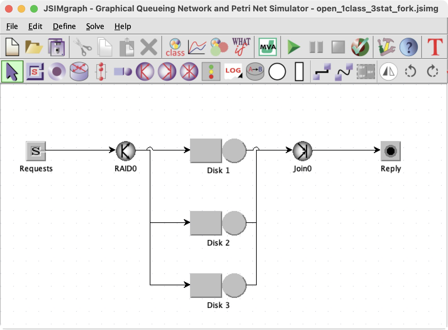
A network needs one or more classes of customers (or jobs or tasks or whatever). Classes were a niche topic in the queue theory book because we usually assumed one class, but classes are a big deal in JMT.
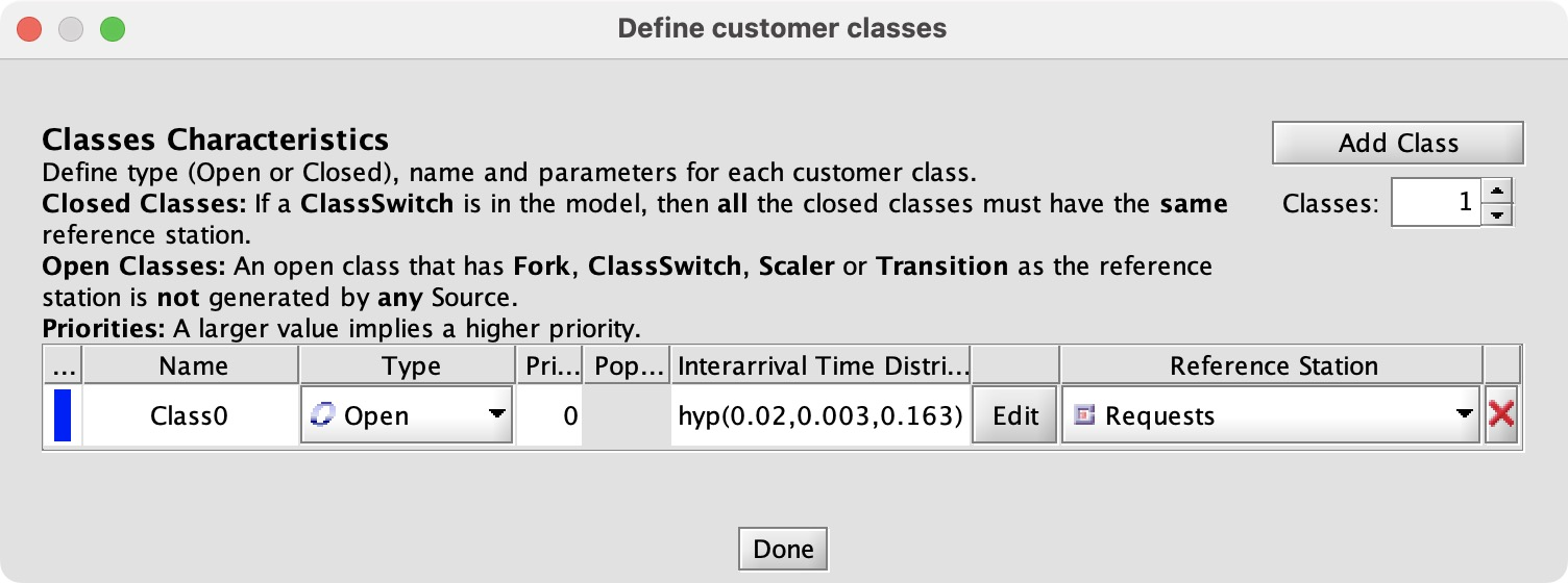
Every class needs a reference station. I have read the manual’s explanation of reference stations five times and I don’t understand, perhaps I need a PhD.
JMT offers a huge number of probability distributions for arrivals, service times, etc. You can choose the “Replayer” distribution which reads values from a file; that could be a trace from your real system or numbers generated by another program.
The goal of running the simulation is to measure some performance indices. Here the indices are the response time for the whole system, and the utilization of each disk.
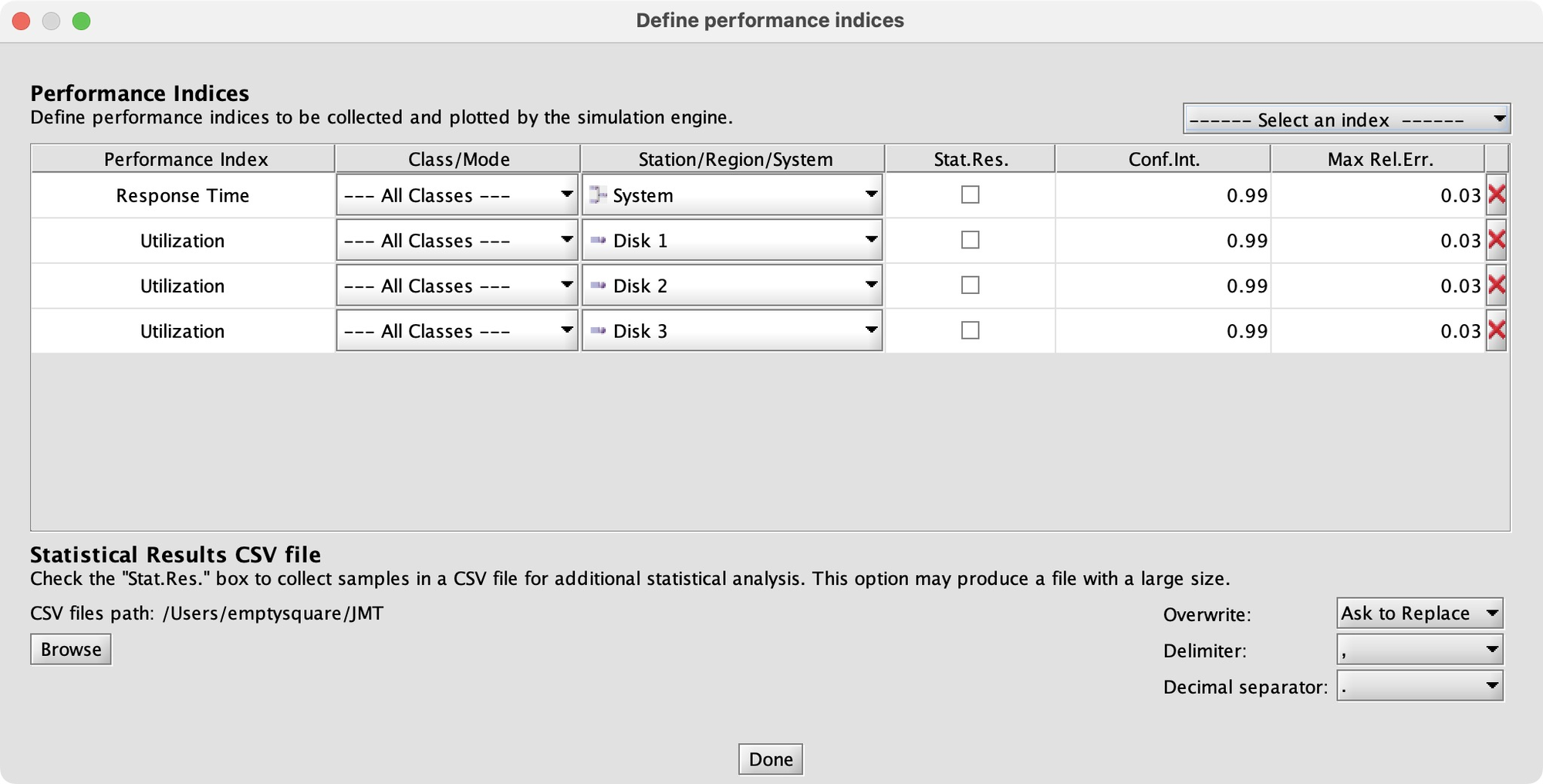
Let’s run the simulation and see those performance indices’ average values:
By default, JSIM runs until each performance index has converged to a stable value within some confidence interval (the red lines converge around the blue lines).
When I showed this to some friends they wondered, “What if the Join0 node waited for a majority of disks instead of all of them?” This was satisfyingly easy to answer. I changed the “join strategy” from “standard” to “quorum”:
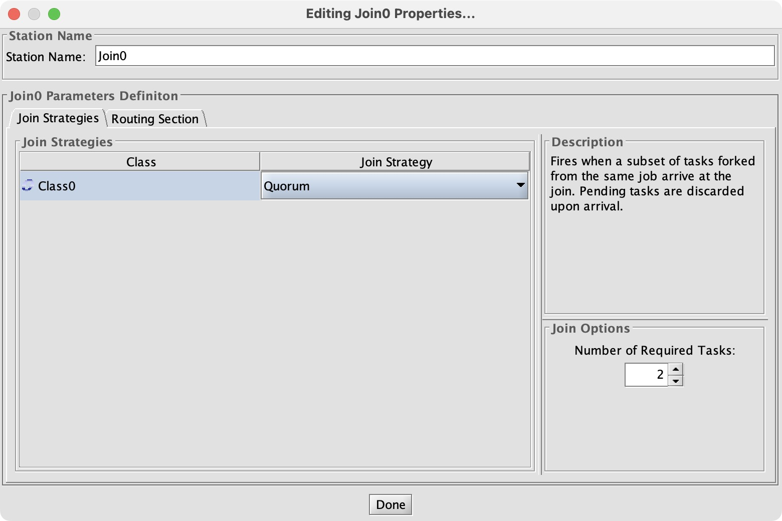
As expected, re-running the simulation shows the same disk utilization but much faster response time: 19 seconds average instead of 34.
Answering a queue theory question #
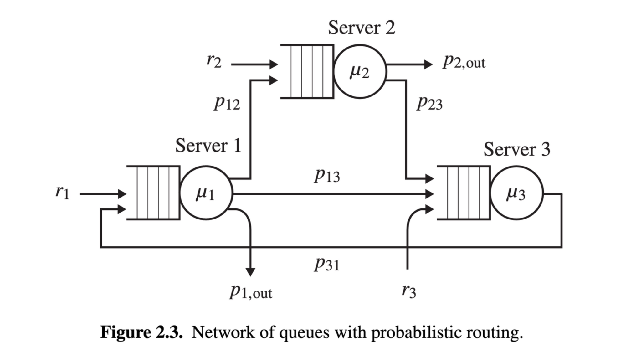
Let’s take a queue theory problem from the book “Performance Modeling and Design of Computer Systems” and contrast the analytic approach to simulation. Here’s a figure from the book:
The book’s Exercise 2.1 asks,
Maximum Outside Arrival Rate
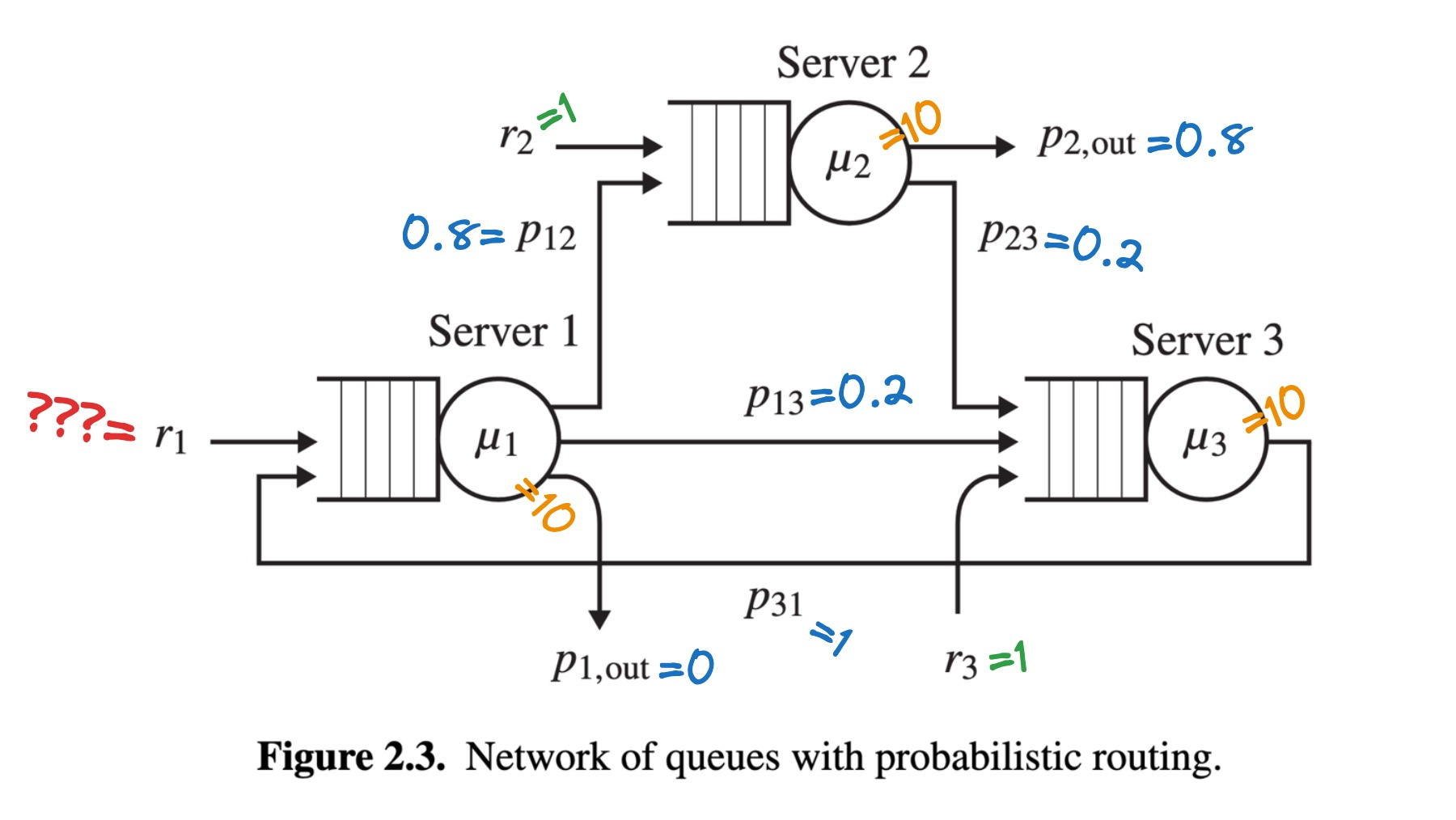
For the network-of-queues with probabilistic routing given in Figure 2.3, suppose that each server serves at an average rate of 10 jobs/sec; that is, μi = 10, ∀i. Suppose that r2 = r3 = 1. Suppose that p12 = p2,out = 0.8, p23 = p13 = 0.2, p1,out = 0, and p31 = 1. What is the maximum allowable value of r1 to keep this system stable?
Let’s add those parameters to the figure:
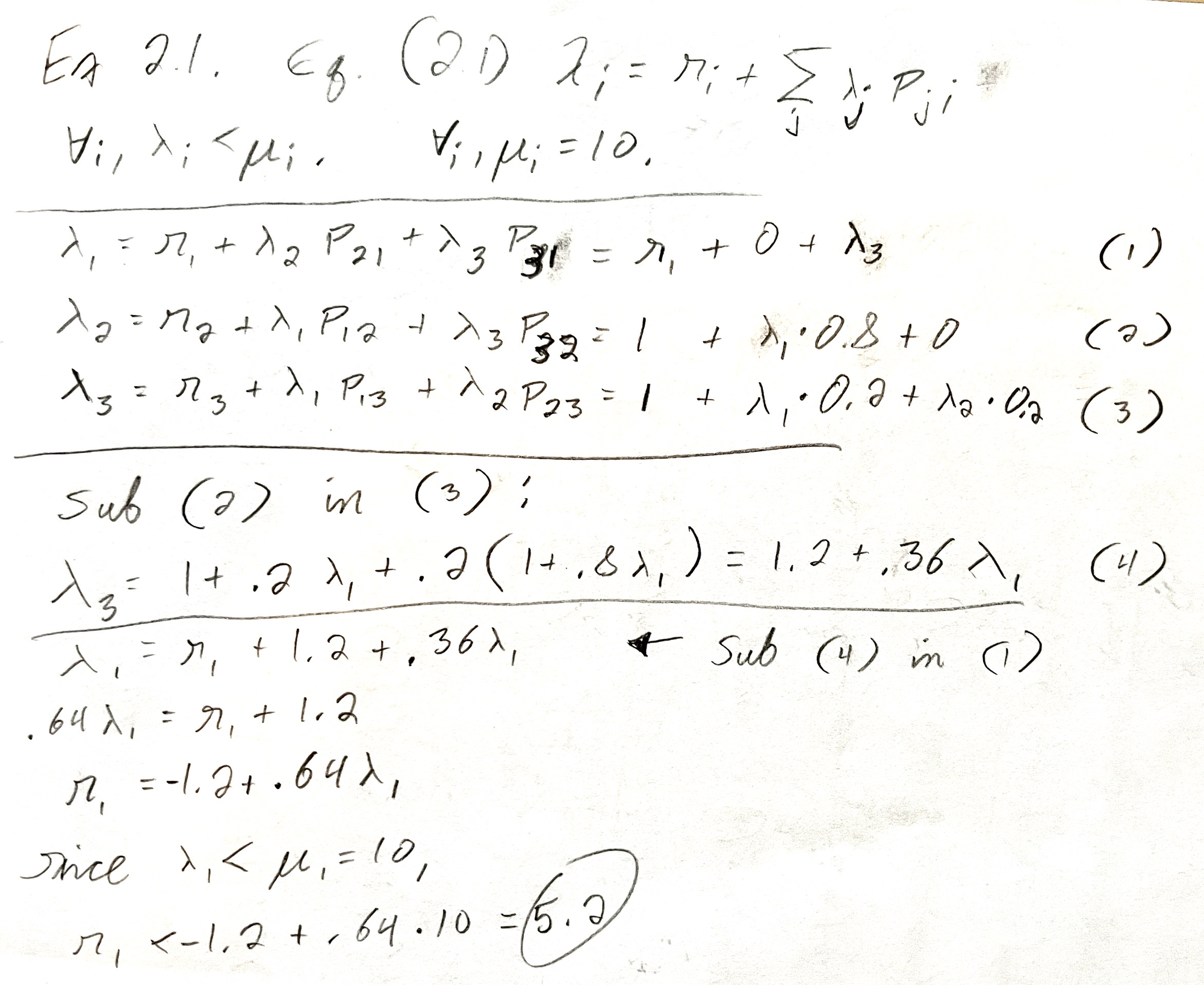
To answer the question, “what’s the max r1”, or “how fast can jobs arrive at Server 1 without overloading the system?”, the book taught me to solve a system of simultaneous equations. I arrived at r1 ≤ 5.2.
I also wrote a 72-line Python simulation (using just the standard library) to confirm this number.
Now that I’ve forgotten how to answer this question with paper and pencil, can I use JMT instead? I drew this uglitude in JSIMgraph:
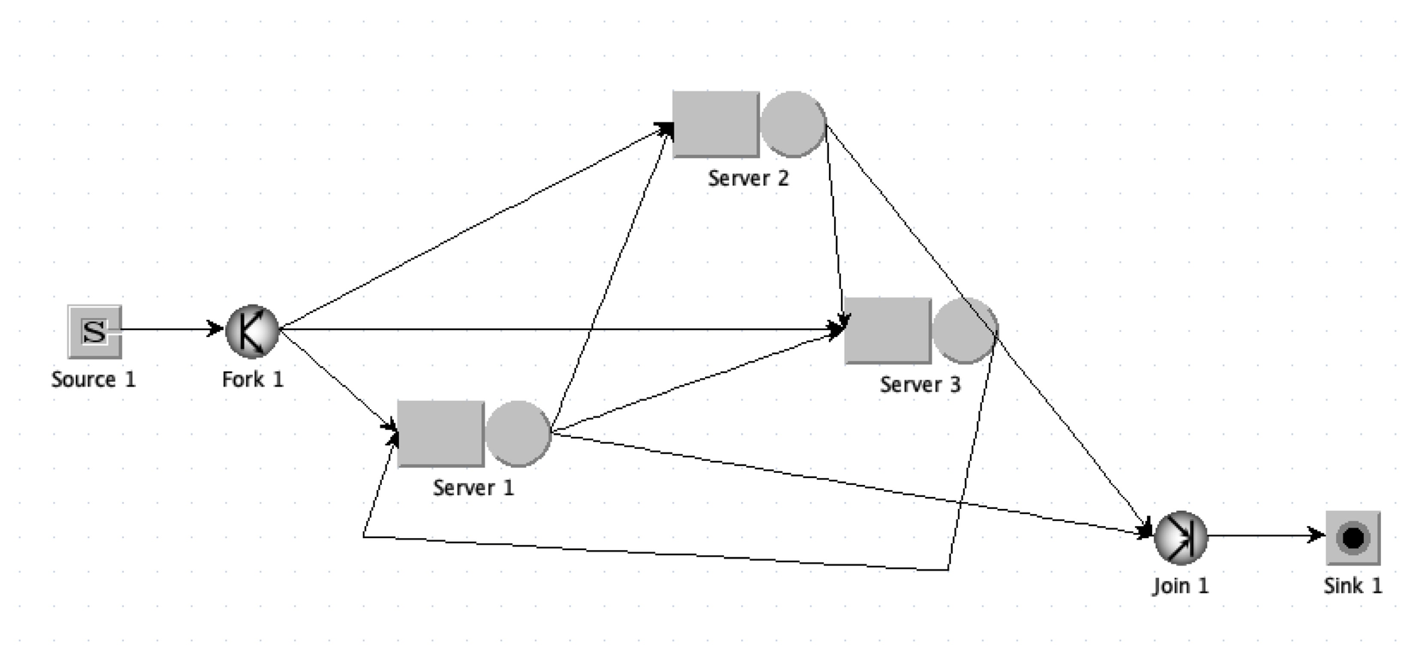
I tried to emulate the book’s figure, with a “source” node for r1, r2, and r3, but this produced strange behavior. Maybe I need to understand “reference stations”. Instead I made three classes of customer (each with a different arrival rate), generated them all at the same source, forked them to the three servers, and collected them in a “sink” node.
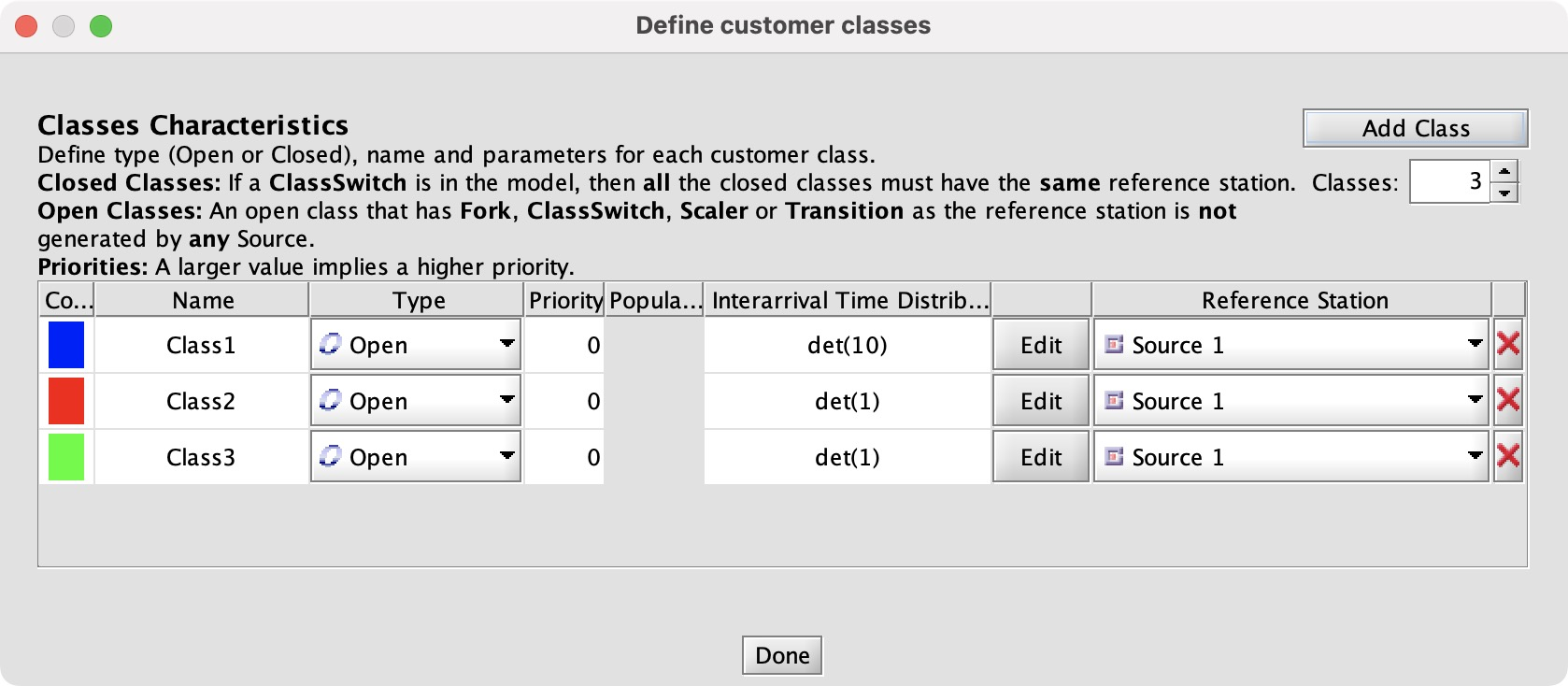
I set Class 1 to 10 arrivals per second, which we know is too high; it should be at most 5.2. The others are 1 per second as in Exercise 2.1. Since we have 3 classes, we have to configure how each server handles each class. First I set the service times to 0.1 for each class (since the exercise says they serve 10 jobs per second), then the routing rules.
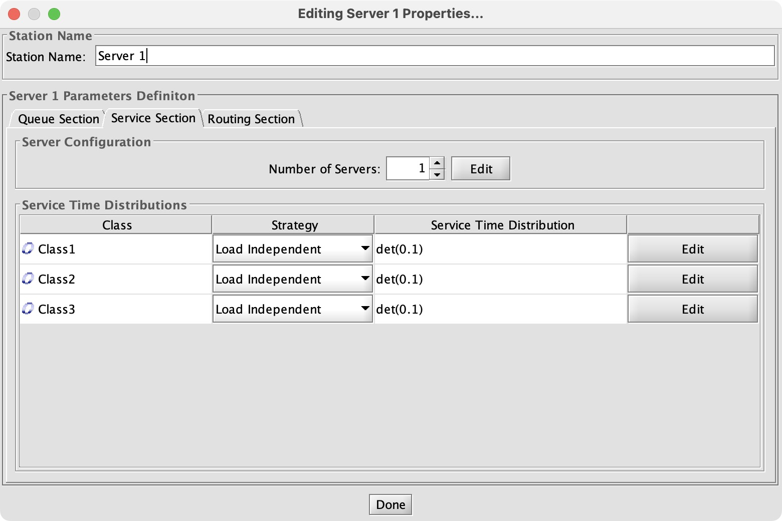
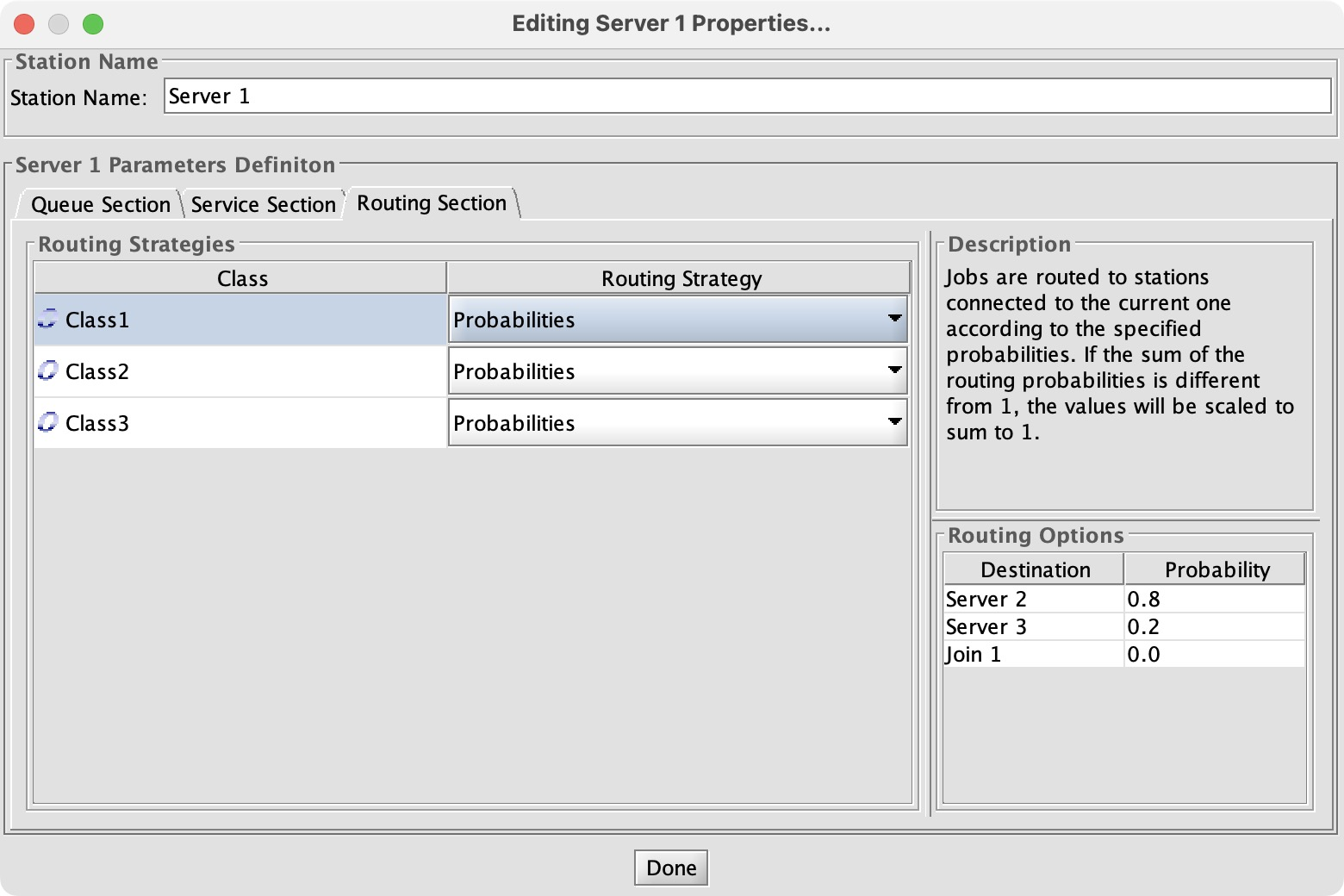
Configuring a queue network is a quickly-growing chore; I have to point and click and enter a number for all classes multiplied by servers multiplied by routes. Worse, there’s no single place to see all the parameters and verify them. I have to double-click each node to open its config dialog, and click among the tabs checking each number.
To find the maximum r1 value I configure a “What-If” analysis, trying a range of values:
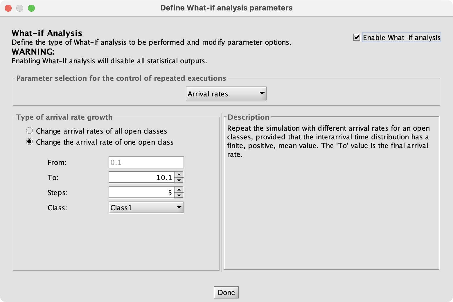
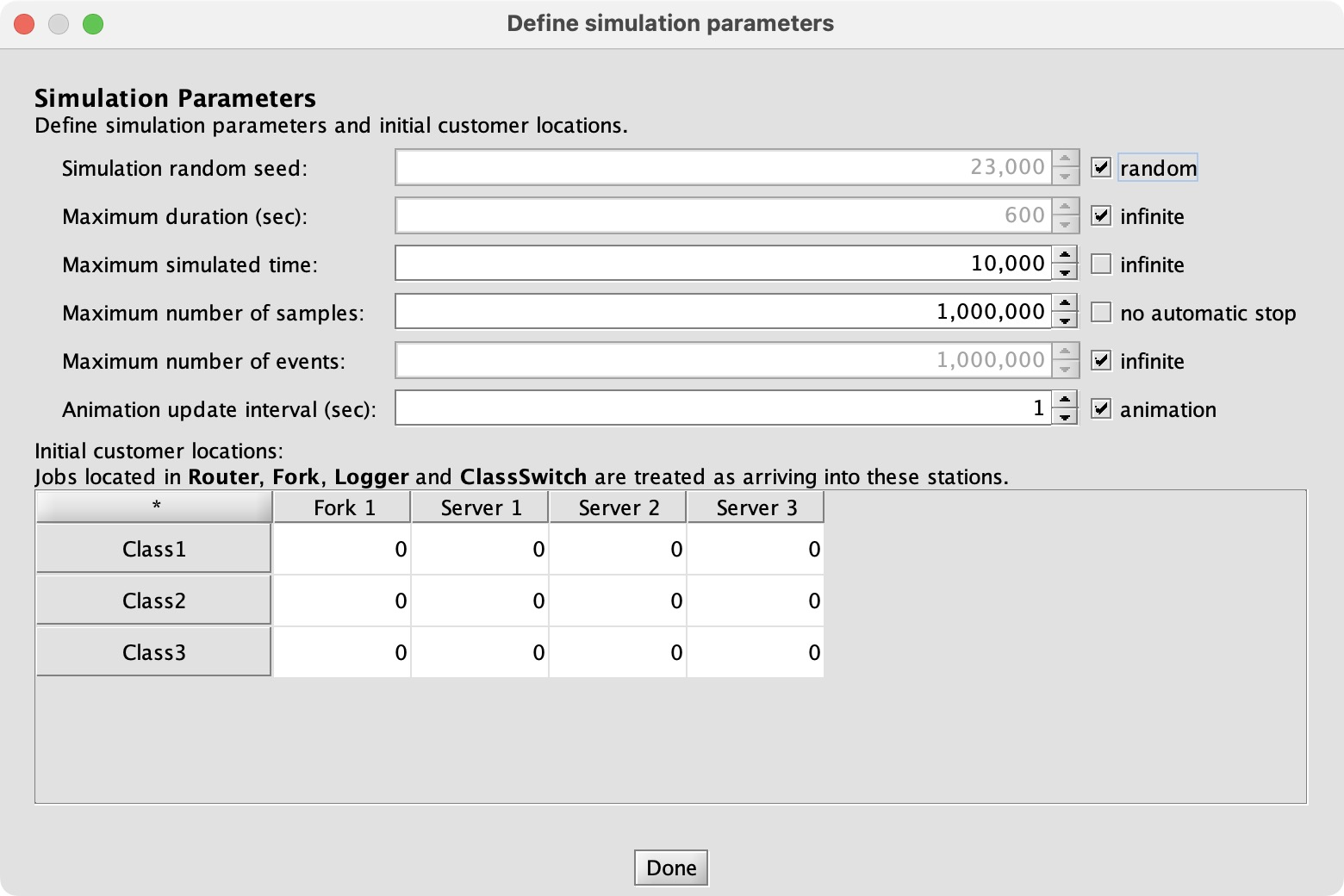
JMT’s simulator assumes by default that the system is stable and its performance indices will converge. In this case, if r1 is too big the system is unstable and JMT runs until it’s out of memory. So I configure the simulation to run for a limited time:
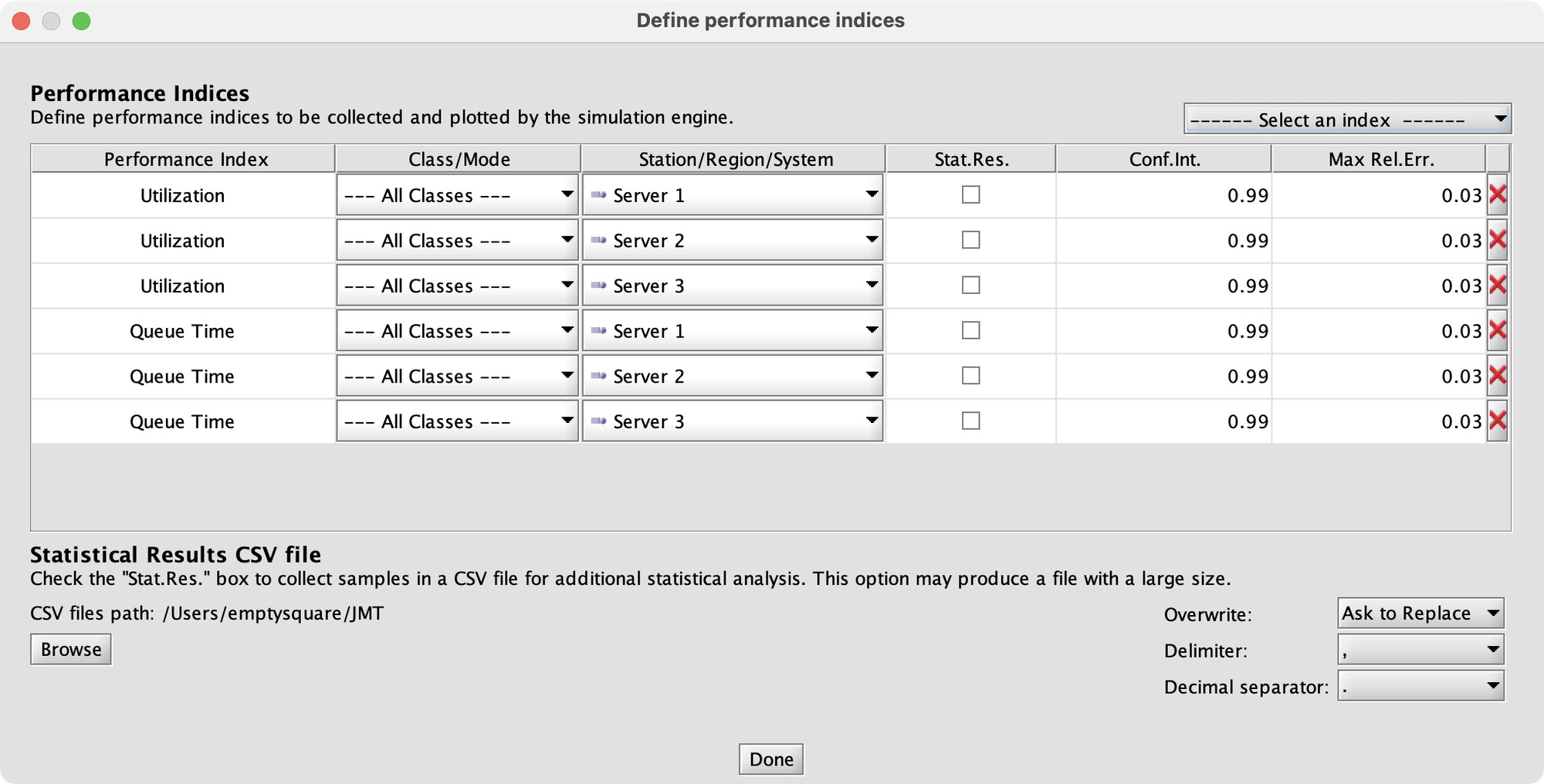
What performance indices will tell me whether the system is stable? If queues grow or a server is fully utilized, those are bad signs, so I’ll measure queueing time and utilization.
Finally, I actually run the analysis:
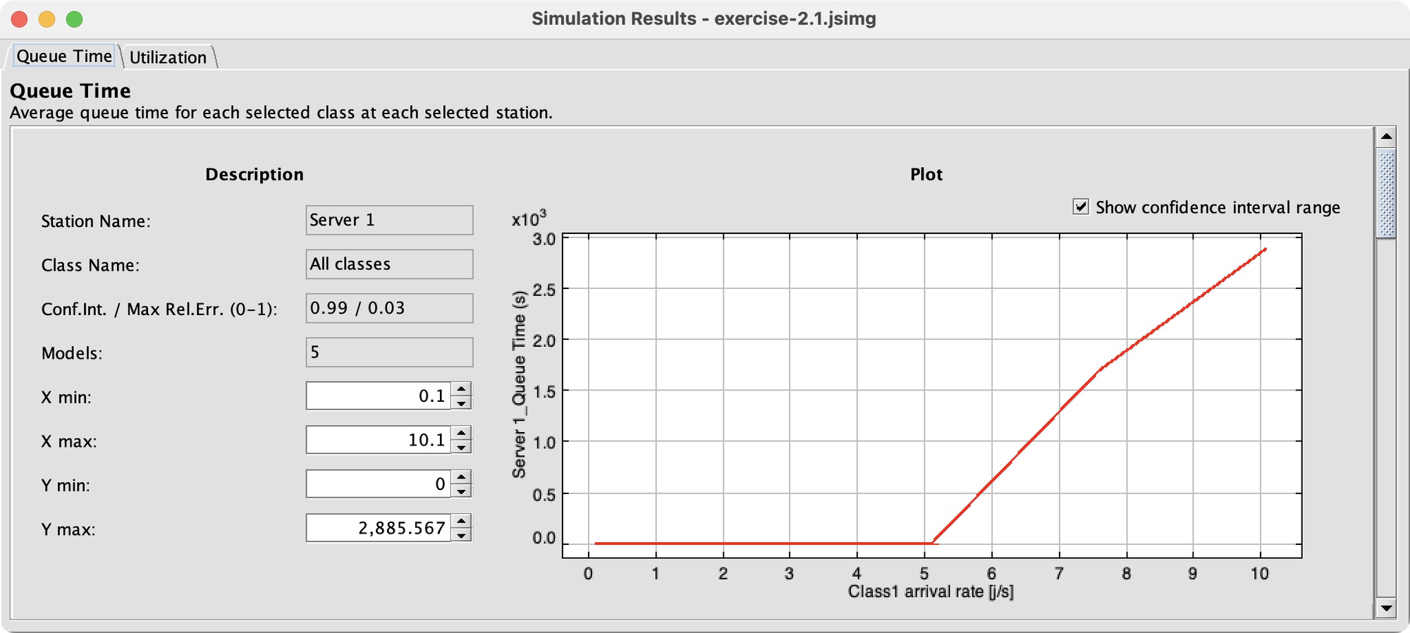
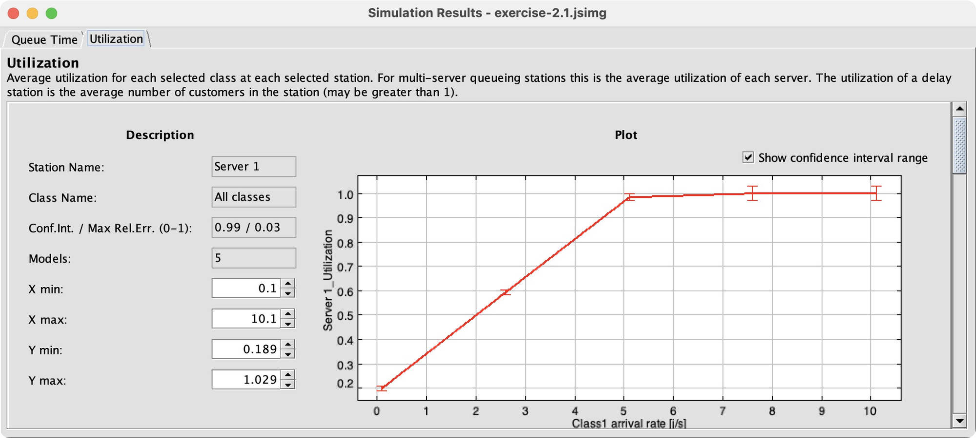
As I had hoped, between the tested r1 values of 5.1 and 6.1, things go haywire. Queueing time takes off and Server 1’s utilization hits 100%. Configuring this was a lot of work, but it’s gratifying to see a clear result. JMT lets me easily measure more performance indices, or tweak the model and see the effects, more easily than in Python and much more easily than paper and pencil.
My evaluation #
Gripes:
- JSIMgraph requires a bunch of pointing, clicking, and typing to set up a queue network with a few classes and nodes. The Python interface looks like a slick way to construct really big networks, but medium networks are a chore.
- Since JSIMgraph expects stable systems by default, doing “what-if” analysis to determine whether a set of params is stable is tricky.
- There’s no single place to see all configuration values, so I have difficulty trusting that I’ve set up a network correctly.
But in JMT’s favor, if your needs fit its features, it’s more convenient than writing a Python simulation, and it overcomes the total impracticality of solving equations. I may play with it some more to learn its features better, and try answering some actual day-job questions about distributed systems.