Are We Serious About Using TLA+ For Statistical Properties?
At this year’s TLA+ community event, I tentatively proposed adding features to make the language useful for performance modeling. Here’s the video, and a written version is below.
Table Of Contents
Half Our Problems #
In 2022, I saw Marc Brooker give a talk called “Formal Methods Only Solve Half My Problems” at HPTS. He published a blog post about this too. He said that TLA+ can check correctness (safety and liveness), but not performance characteristics. “What I want is tools that do both: tools that allow development of formal models … and then allow us to ask those models questions about design performance.” He acknowledges that correctness is important. But it’s not enough to say nothing bad ever happens, and something good eventually happens—we want to know how quickly something good happens!
How would we actually create such a tool? Marc said that queueing theory was the kind of math that was obviously useful for this.
Learn Queueing Theory? #
So I decided to learn queueing theory. I asked Marc what book I should read, and he recommended Performance Modeling and Design of Computer Systems, Queuing Theory in Action. The title sounds like it’s the perfect book for our purposes, so I recruited Andrew Helwer and Murat Demirbas to read it with me. We spent 8 months reading most of the book and doing a lot of the problem sets. It was definitely interesting, but mostly irrelevant to the actual problem of, you know, performance modeling and design of computer systems.
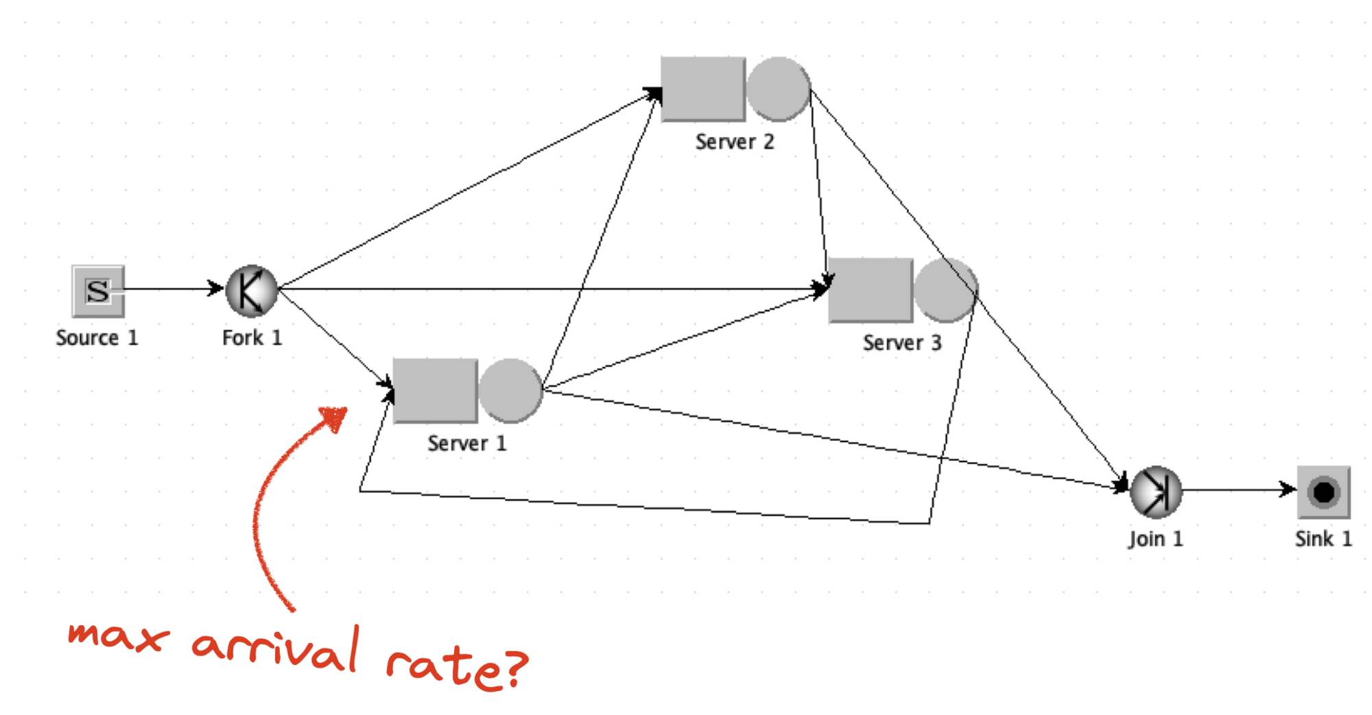
As an example of a queueing theory problem, here’s a diagram from Chapter 2 of the book.
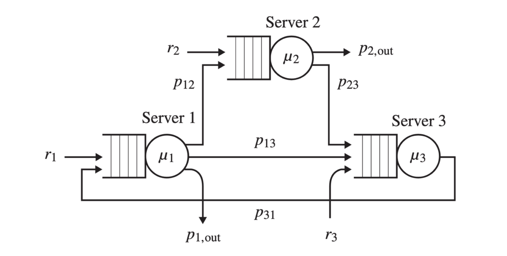
There are three servers, each with a queue where tasks arrive. A server processes tasks from its queue, and then the task either leaves the network, or it gets sent to another server’s queue. There are probability distributions for all these events: the delays between task arrivals, the time it takes for a server to process a task, the chance a task leaves the network or goes to another server.
What kinds of questions does queueing theory answer about this system?
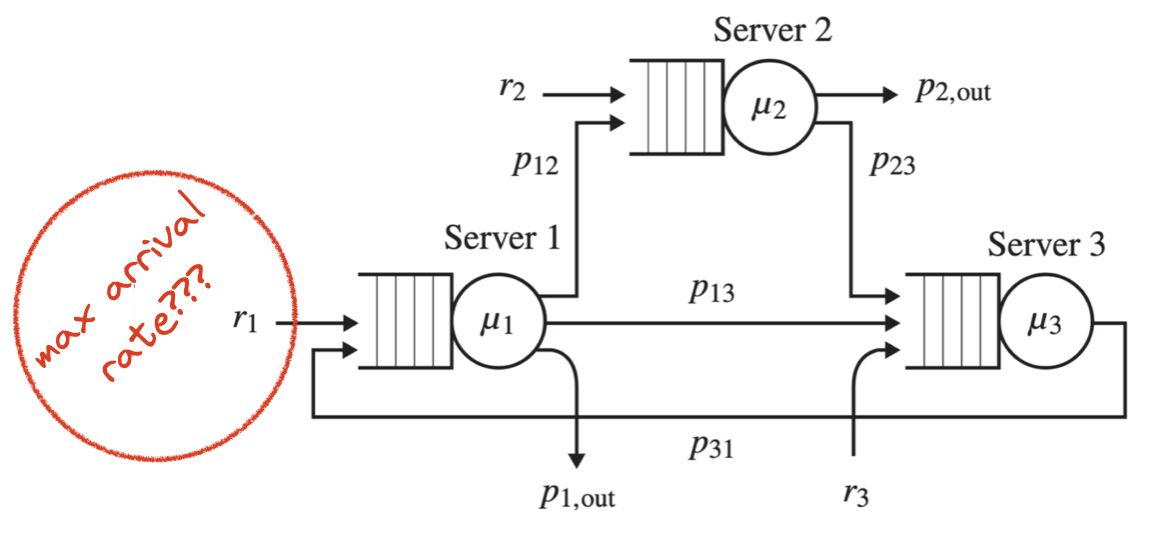
In the book, one of the exercises asks a classic queueing theory question, which is also a practical question: what’s the maximum arrival rate at Server 1’s queue that the system can handle?
I did my homework with paper and pencil. I solved some equations using the techniques in the book and came up with an answer: the max arrival rate is 5.2.
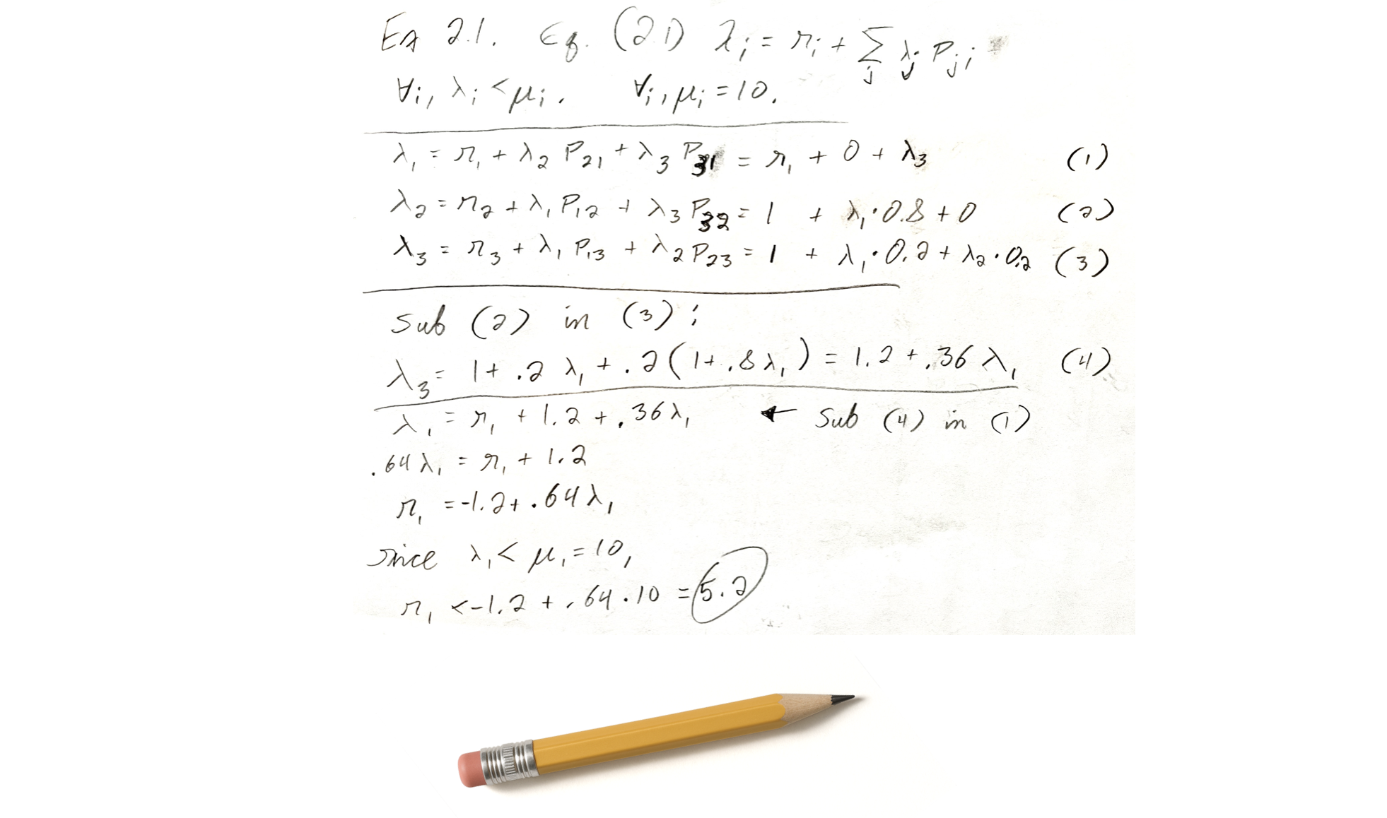
I don’t think we should try to answer performance questions by writing equations and solving for a variable! It’s hard to get right, easy to get wrong, and you have to recalculate every time the inputs change. I think we should just use simulation—run an experiment thousands of times and take the average. Call it “Monte Carlo” simulation if that makes you feel better.
Java Modelling Tools #
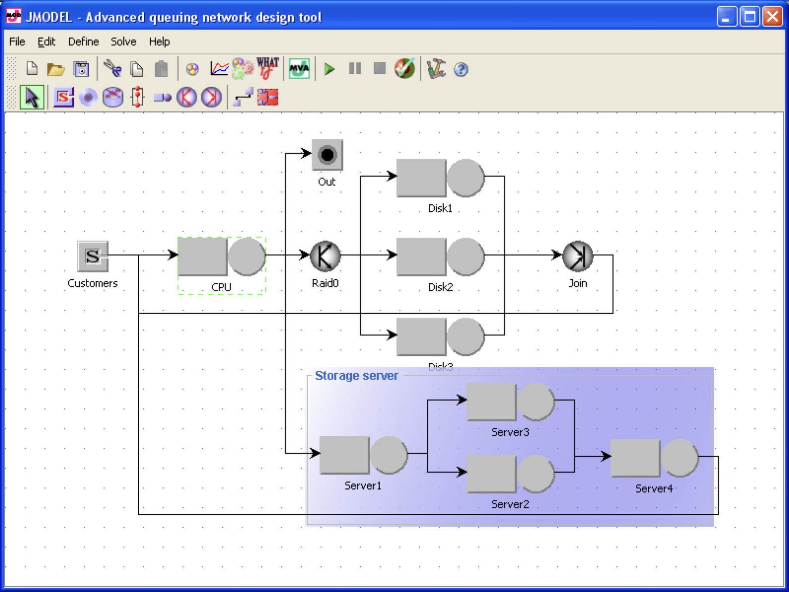
There’s an open source toolkit that will do this for you, an academic project called the Java Modelling Tools. They’re a bunch of tools for modeling queue networks and then answering questions about them, through some combination of equation-solving and simulation. I started from the exercise in the book, and I used JMT to draw this very ugly version of the same queue network:
I configured a bunch of things and ran a simulation where I varied the arrival rate at Server 1:
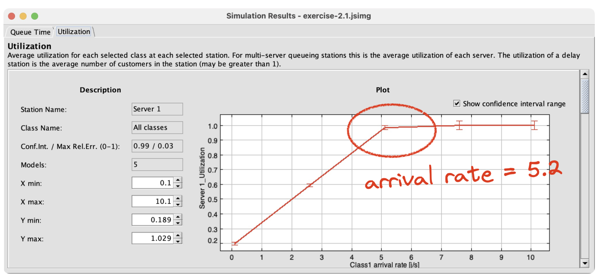
JMT lets me sweep the value of the arrival rate from 0 to 10 by increments of 0.1—that’s the independent variable—and I can simulate the system and measure the server utilization that results—that’s the dependent variable. You can see that when the arrival rate reaches 5.2, server utilization reaches 1.0, meaning it’s completely utilized and the system has reached its capacity. That’s the answer I got with my pencil, too. This kind of simulation works even for complex queue networks where the math is hard or impossible.
What I’ve learned from the book and the tool is that queueing theory has super-useful concepts: arrival rate, service rate, utilization, ergodicity, Little’s Law, service discipline, open vs. closed loop, and many more. But the math is heinous. There are some simple equations to start you off, like Little’s Law, and then all hell breaks loose. So, don’t try to learn the math. No matter how good you are at math, queueing theory math won’t get you what you want. Specifically, you’ll never be able to estimate system performance by solving equations. You can only solve the equations for extremely simple systems. If you want to model a real-world system, the math will be an open research question, or literally impossible.
If we use simulated queue networks to model performance, have we solved both Marc’s problems? No, Marc wants one tool that both checks an algorithm’s correctness and models its performance, with a single specification.
TLA+ for Performance Modeling #

The same year Marc talked about this, Jack Vanlightly and Markus Kuppe presented “Obtaining Statistical Properties via TLC Simulation.” They described how to write a spec and use TLC to measure statistics. (Video, slides, Jack’s article, Murat’s review.) I’ll show some code examples from Jack’s spec for a gossip protocol.
\* Increment the updates counter by the number of incoming peer states.
TLCSet(updates_ctr_id, TLCGet(updates_ctr_id)
                       + Cardinality(DOMAIN incoming_peer_states))
The spec uses TLCSet to record each statistic. Here it’s counting the number of times nodes get new information. TLCSet and TLCGet access a global scratchpad, so you can record things outside of the state space.
CSVWrite(
  "%1$s,%2$s,%3$s,%4$s,%5$s,%6$s,%7$s,%8$s,%9$s,"
  \o "%10$s,%11$s,%12$s,%13$s,%14$s,%15$s,%16$s,"
  \o "%17$s,%18$s,%19$s,%20$s,%21$s,%22$s,%23$s,"
  \o "%24$s,%25$s",
  <<behaviour_id,
    r, RoundMessageLoad(r), DirectProbeDeadMessageLoad(r),
    IndirectProbeDeadMessageLoad(r), TLCGet(updates_pr_ctr(r)),
    TLCGet(eff_updates_pr_ctr(r)),
    alive_count, suspect_count, dead_count, alive_states_count,
    suspect_states_count, dead_states_count,
    infective_states_count, infectivity, cfg_num_members,
    cfg_dead_members, cfg_new_members, SuspectTimeout,
    DisseminationLimit, cfg_max_updates, cfg_lose_nth,
    cfg_peer_group_size, cfg_initial_contacts, MaxRound>>,
  RoundStatsCSV)
This code appends a line to the CSV file, recording the results of the execution. Jack had to hand-code this in TLA+, and hand-code the logic for when to run this during TLC’s execution, and so on. It’s impressive that it works at all, but it’s kind of a hack.
So my Complaint Number 1 is the syntax. What we have now in TLA+ is hard to write, it attracts bugs, and it clutters up the specification.
\*  'probabilistic' is a random chance of losing the message
\*  'exhaustive' is for model checking where both options are explored
GetDeliveredCount() ==
  CASE MessageLossMode = "probabilistic" ->
      IF RandomElement(1..cfg_lose_nth) = cfg_lose_nth
      THEN {0}
      ELSE {1}
    [] MessageLossMode = "exhaustive" -> {0,1}

SendMessage(msg) ==
  \E delivered_count \in GetDeliveredCount() :
    \* ... send the message if delivered_count is 1 ...
Here’s some code to determine whether a message is delivered or lost. Jack has a config option called MessageLossMode, he has to set it to “probabilistic” to make statistics work, or set it to “exhaustive” to make model-checking work. My Complaint Number 2 is that randomization is incompatible with model-checking and you have to code workarounds. (Correction: Markus says this is fixed now!)
Jack has another a constant called cfg_lose_nth, let’s say it’s 4, then in probabilistic mode there’s a one-in-four chance that a message is lost. You could extend this to any rational number, like two-out-of-three, but you can’t work with irrational numbers. TLC doesn’t have floating-point numbers at all. So my Complaint Number 3 is that randomization is very limited. It’s just Dungeons & Dragons dice throws.

If you want to measure performance, you need some sort of cost function. E.g., sending a message to Tokyo might cost 2.5 times as much as sending it to London. Or its cost might be exponentially distributed. Here’s some imaginary TLA+ for accumulating the cost of an algorithm:
\* In your dreams
TLCSet(cost, TLCGet(cost) + 1.0)
TLCSet(cost, TLCGet(cost) + 2.5)
TLCSet(cost, TLCGet(cost) + Exponential(3))
All the examples I’ve seen of statistical properties in TLA+ are counting the number of times some discrete event occurs, like counting the number of messages. But if we want to measure the performance of a system as a whole, we need to measure a variety of events, and they have to have relative costs! Complaint Number 4 is we have no floats and no probability distributions besides “uniform”.
Statistical Properties in TLA+, So Far #
I think it’s just a proof of concept. Jack and Markus’s technique works and it’s useful. What they accomplished is impressive and it started the conversation. But it’s insufficient if we’re serious about using TLA+ for statistics. TLCSet and the CSV module provide a manual, low-level API to save statistics. Compared to safety and liveness checking, which are first-class features of the language and tools, statistical modeling really clutters up the specification.
As we saw with Jack’s gossip protocol, it’s not only a large amount of code, but it’s error-prone, you have to write it into each spec, and you don’t get the benefit of a tested and documented library. People need a concise and easy API for saving statistics.
The Randomization module only gives us uniform distributions with integer parameters. Performance modeling requires lots of distributions, such as Poisson, exponential, and Zipf. Limiting probabilities to ratios of integers is an artifact of our unfinished tooling; we should give TLA+ authors the freedom to choose whatever probabilities they want.
If you want to model the performance of a whole system, you need to combine the costs of different actions. You can do that manually with TLCSet, but there’s no standard convenient way to do it.
And there are no floats. This makes sense for model-checking, but it’s a silly limitation for performance modeling. I’ll stop talking about that before I get too annoying.
Statistical Properties: Are We Serious? #
So, what we have right now in TLA+ isn’t really solving both of Marc’s problems. Should we try? Should TLA+ be the tool that solves both, or should we stay focused on safety?
I don’t know. I haven’t implemented anything, I’m just offering ideas. And I want to admit I’m not offering any time or money to this project, so I can’t make any demands. I’m just brainstorming with you.
State of the Art #
As a start, let’s look at some existing tools: JMT, PRISM, Runway, and FizzBee.
State of the Art #1 of 4: Java Modelling Tools #
We saw JMT above; it’s the tool where you can draw queue networks. It’s made for statistical modeling and answering performance questions. It has a point-and-click interface, which is good for small models and bad for big ones. There’s also a Python API for generating large models. It comes with lots of probability distributions built-in, it can model cost functions, and you can use real-world data sets as inputs! E.g., if you have some data about the distribution of network latencies, you can import that into a JMT model.
State of the Art #2 of 4: PRISM #
PRISM is built for exactly this problem. It’s a “probabilistic model checker”: you write a spec of an algorithm and ask statistical questions, like the probability of something happening, or the average cost.
Actions in PRISM look like this:
[my_action] x=0 -> 0.8:(x'=1) + 0.2:(x'=2);
You have an action name (“my_action”), a guard, which is some predicate (this action is enabled if x is zero), and some state updates with probabilities. There’s a 0.8 probability that it sets x to 1 and a 0.2 probability that it sets x to 2. These numbers are either probabilities that something happens, or the rates at which things happen, depending on whether you’re writing a discrete-time or continuous-time model.
PRISM has built-in support for cost functions. A cost is just anything you want to measure, any way of expressing performance. PRISM calls costs “rewards,” but if you’re thinking of reinforcement learning, stop. This is not related to reinforcement learning.
rewards
    x=0 : 100;
    x>0 & x<10 : 2*x;
endrewards
This code says that every state where x equals zero has a reward of 100, and if x is between 0 and 10 then the reward is twice x. You can imagine writing a reward function that measures revenue, or a reward function that’s actually a cost function that measures something bad, like latency.
PRISM has remarkably powerful property expressions. Here’s an example from their website, it’s “the probability that more than 5 errors occur within the first 100 time units is less than 0.1.” This is an assertion that PRISM checks.
P<0.1 [ F<=100 num_errors > 5 ]
Here’s another, “the probability that process 1 terminates before process 2 does.” This is a question—what is the probability?—and PRISM will give you the answer.
P=? [ !proc2_terminate U proc1_terminate ]
You could express safety as an assertion: the probability of something bad happening is zero. Liveness is an assertion that the long-run probability of something good happening is 1. But there are much more complex and powerful probabilistic properties you can express and check in PRISM, like saying that the 95th-percentile latency of an algorithm is less than some acceptable amount.
The PRISM website has a bunch of great examples. Here are statistics from a PRISM model of a gossip protocol. As nodes discover each other over time, they find shorter paths from node to node:

This kind of analysis and graphing is built into PRISM, it was born for this.
PRISM can only express models that are simple enough to analyze by solving equations. So the PRISM language has no arrays, no hashtables, no sets. It’s just scalar variables with float values, pretty much. That makes PRISM specs kind of awful.
Here’s the PRISM gossip protocol. This model has 4 nodes. Each node’s view of each other node is a separate variable, so that’s 16 variables:
// initial view of node 1 (can see 2 one hop away)
const int iv1_1_a = 2;
const int iv1_2_a = 0;
const int iv1_1_h = 1;
const int iv1_2_h = 4;

// initial view of node 2 (empty)
const int iv2_1_a = 0;
const int iv2_2_a = 0;
const int iv2_1_h = 4;
const int iv2_2_h = 4;

// initial view of node 3 (can see 2 one hop away)
const int iv3_1_a = 2;
const int iv3_2_a = 0;
const int iv3_1_h = 1;
const int iv3_2_h = 4;

// initial view of node 4 (can see 2 one hop away)
const int iv4_1_a = 2;
const int iv4_2_a = 0;
const int iv4_1_h = 1;
const int iv4_2_h = 4;
If you had 5 nodes, you’d need 25 variables. You can’t write any generic code. As the number of nodes grows, the code in this spec grows. This is Node 1’s code for talking to Nodes 2, 3, and 4:
// send to node 2
[push1_2_0] s1=3 & send1=id2 & i1=0 -> (i1'=i1+1);
[push1_2_1] s1=3 & send1=id2 & i1=1 & v1_1_h<4 -> (s1'=0) & (i1'=0) & (send1'=0);
[push1_2_end] s1=3 & send1=id2 & ((i1=1&v1_1_h=4) | (i1=2&v1_2_h=4)) -> (s1'=0) & (i1'=0) & (send1'=0);
// send to node 3
[push1_3_0] s1=3 & send1=id3 & i1=0 -> (i1'=i1+1);
[push1_3_1] s1=3 & send1=id3 & i1=1 & v1_1_h<4 -> (s1'=0) & (i1'=0) & (send1'=0);
[push1_3_end] s1=3 & send1=id3 & ((i1=1&v1_1_h=4) | (i1=2&v1_2_h=4)) -> (s1'=0) & (i1'=0) & (send1'=0);
// send to node 4
[push1_4_0] s1=3 & send1=id4 & i1=0 -> (i1'=i1+1);
[push1_4_1] s1=3 & send1=id4 & i1=1 & v1_1_h<4 -> (s1'=0) & (i1'=0) & (send1'=0);
[push1_4_end] s1=3 & send1=id4 & ((i1=1&v1_1_h=4) | (i1=2&v1_2_h=4)) -> (s1'=0) & (i1'=0) & (send1'=0);
Node 2 borrows Node 1’s code by horribly renaming all its functions:
push1_2_0=push2_1_0, push1_2_1=push2_1_1, push1_2_2=push2_1_2, push1_2_3=push2_1_3, push1_2_end=push2_1_end,
push1_3_0=push2_3_0, push1_3_1=push2_3_1, push1_3_2=push2_3_2, push1_3_3=push2_3_3, push1_3_end=push2_3_end,
push1_4_0=push2_4_0, push1_4_1=push2_4_1, push1_4_2=push2_4_2, push1_4_3=push2_4_3, push1_4_end=push2_4_end,
push2_1_0=push1_2_0, push2_1_1=push1_2_1, push2_1_2=push1_2_2, push2_1_3=push1_2_3, push2_1_end=push1_2_end,
push3_1_0=push3_2_0, push3_1_1=push3_2_1, push3_1_2=push3_2_2, push3_1_3=push3_2_3, push3_1_end=push3_2_end,
push4_1_0=push4_2_0, push4_1_1=push4_2_1, push4_1_2=push4_2_2, push4_1_3=push4_2_3, push4_1_end=push4_2_end
I’m only showing you a fraction of this code to preserve your sanity. Nodes 2 and 3 have the same kind of thing. This is an abomination. This code is banned by the Geneva Convention. The grad student who wrote this code was found lying on the floor of the computer science lab, drooling.
Actually it was probably generated by a program in another language. PRISM is like an assembly code for expressing Markov chains. This makes it tractable for PRISM’s equation solver to come up with exact solutions, but it’s obviously not a good language.

Start of the Art #3 of 4: Runway #
In 2016, Diego Ongaro announced a formal modeling system called Runway (website, article, Andrew’s summary.) Ongaro had published Raft a couple years before, then he announced this very promising-looking thing but stopped working on it the same year. This is a snippet from a Runway specification of Raft.
function quorum(serverSet: Set<ServerId>[ServerId]) -> Boolean {
  return size(serverSet) * 2 > size(servers);
}

function sendMessage(message: Message) {
  message.sentAt = later(0);
  message.deliverAt = later(urandomRange(10000, 20000));
  push(network, message);
}
Runway’s syntax is familiar for programmers. And Runway has randomization built in. If Runway is in model-checking mode, it somehow tries all possibilities; I don’t know how. If Runway is in simulation mode, randomization works the way you’d expect, and Runway can gather statistics.
Here’s an elevator simulation written in Runway:
The visualization on the right needs lots of custom code, but the graph on the left is I think easy to create with Runway’s built-in tools. If we want to develop TLA+ tools in this direction, we should make this kind of graph convenient for spec authors to generate.
State of the Art #4 of 4: FizzBee #
FizzBee is a new modeling language developed by a solo author, Jayaprabhakar “JP” Kadarkarai. Here’s an example FizzBee spec from the FizzBee docs:
| cache.fizz | perf_model.yaml |
atomic action Lookup:
  cached = LookupCache()
  if cached == "hit":
      return cached
  found = LookupDB()
  return found


func LookupCache():
  oneof:
    `hit` return "hit"
`miss` return "miss" |
configs:
  LookupCache.call:
    counters:
      latency_ms:
        numeric: 10
  LookupCache.hit:
    probability: 0.2
  LookupCache.miss:
probability: 0.8 |
The spec describes a service that tries to look up data in a cache, then falls back to a database query. The algorithm is in cache.fizz on the left; Lookup and LookupCache are defined there. (I omitted LookupDB.) On the right is a config file that’s only for probabilistic modeling! It defines the cost of a call to the LookupCache function: 10 milliseconds of latency. PRISM avoids the valenced “cost” / “reward” terms and calls this value a “counter”, but it can be a float. Counters and probabilities are kept in this separate config file. They don’t clutter the spec, and they’re not needed for ordinary model-checking (i.e. checking safety properties).
The LookupCache function is nondeterministic, it either finds the data or doesn’t. The transitions are labeled as `hit` or `miss` in the spec, and their probabilities are defined as 0.2 and 0.8 in the config file. Again, the algorithm is kept separate from the probabilistic config.
FizzBee’s probabilistic modeler, a.k.a. the performance model checker, is a separate program from the safety model-checker. The former produces the state graph and saves it to disk; the latter reads the state graph and produces statistics. If you run the performance modeler on the files above, it prints:
Metrics(mean={'latency_ms': 84.4}, histogram=[(0.2, {'latency_ms': 10.0}), (1.0000000000000002, {'latency_ms': 103.0})])
   2: 0.20000000 state: {} / returns: {"Lookup":"\"hit\""}
   4: 0.72000000 state: {} / returns: {"Lookup":"\"found\""}
   5: 0.08000000 state: {} / returns: {"Lookup":"\"notfound\""}
The mean latency to look up one value is 84.4, and the return value of Lookup is “hit” 20% of the time, “found” 72% of the time, and “notfound” 8% of the time, as we’d expect from the defined probabilities.
Here’s the config file again, but with a probability distribution for the cost function.
perf_model.yaml
configs:
  LookupCache.call:
    counters:
      latency_ms:
        distribution: lognorm(s=0.3, loc=2)
FizzBee lets you choose any probability distribution supported by SciPy, which is basically all of them. Or you can bring your own histogram of costs: if you have experimental data, you can use that, the same as with the Java Modelling Tools. Marc Brooker said he wants a tool that uses “real-world data on network performance, packet loss, and user workloads,” and FizzBee allows this.
I think FizzBee’s design is smart. FizzBee has built in some important ideas: cost functions, probability distributions, and probabilities of state transitions. We don’t have to write a bunch of error-prone code for each spec, the batteries are included. What’s really nice is that the performance stuff is all in a separate file, so it doesn’t clutter the main spec. In TLA+ we try to keep model-checking details out of the main spec; FizzBee lets you do the same with performance modeling.
I don’t know how much of this is implemented. FizzBee is new and JP has been developing it solo. But that’s not important because we’re just gathering design ideas for what TLA+ might do.
A Menu for TLA+ #
I’ve grouped the features we’ve seen so far into three categories:

Some of the state-of-the-art tools can annotate state transitions with probabilities. Some support cost / reward functions, which FizzBee calls “counters”. PRISM has powerful statistical property expressions. In Runway and FizzBee, model-checking is compatible with performance modeling (and now TLA+ too), and FizzBee nicely separates performance modeling config. Some include convenient charting. They all support floating-point numbers. Some of them ship with common probability distributions for rates and cost functions. Some can use experimental data as a probability distribution (“bring your own histogram”). Some of them come with solvers that calculate answers precisely, but this limits the models to those that can be solved in closed form. Others use statistical sampling, which is imprecise but much more powerful.
Possible Syntax?? #
Here’s the moment I dread, when I suggest a syntax. Everywhere a spec has nondeterminism for model-checking, we need to replace that with some sort of probability distribution. E.g., this formula picks an element nondeterministically from a set:
\* MySpec.tla
SendMessage(m) ==
  \E messageIsDropped \in {FALSE, TRUE}:
    ...
If you want a distribution besides uniform, you could wrap the set (or any collection) in an operator like this:
\* MySpec.tla
SendMessage(m) ==
  \E messageIsDropped \in MessageLossProbability(FALSE, TRUE):
    ...
The operator does nothing in model-checking mode, but it’s like a label for a probability distribution.
\* MySpec.cfg
DISTRIBUTION
  MessageLossProbability = BooleanChoice(0.23)
In the config file, labeling this operator as a DISTRIBUTION means the model-checker treats it as either true or false, and it explores both possibilities nondeterministically. The performance-modeler knows that this is a particular probability, perhaps BooleanChoice is the name of a built-in utility to return its first argument with probability 0.23, otherwise its second argument. Like FizzBee, we use labels to tie the spec to the configuration.
We also need cost functions in TLA+. We could set the cost of each action to be a constant or a probability distribution. The distribution could come from real-world data, and it could be parameterized if the action is parameterized.
\* MySpec.cfg
COST
  SendMessage = Exponential(3.17)
This is the part of my talk I’m least sure about. If you hate this syntax, that’s fine, don’t get angry at the whole idea because you hate my syntax.
TLA+ with Probabilistic Solvers #
If we implement any of this in TLA+, we’ll need some way to actually answer these probabilistic questions. In order of ambitiousness:
- Just use TLC’s -generate option, generate thousands of behaviors, average the stats.
- Use -generate, run until stats stabilize within some precision. Perhaps prune branches of the state graph as they stabilize. JMT does similar smart exploration of simulations.
- Use PRISM’s solvers, by translating the state graph to PRISM code, or otherwise borrowing PRISM’s implementation.
- Write a solver or solvers from scratch: translate the state graph to a Markov chain and find its steady-state probability distribution.
The latter two options will find closed-form solutions with precise answers, but severely limit our options for what models we can use for probabilistic questions. I think we should just use simulation, period.
TLA+ with Performance Modeling #
If we actually had TLA+ with performance modeling, it could be really cool! One model could:
- Express the algorithm.
- Check correctness.
- Evaluate performance.
- Simulate “what-if” experiments using real-world inputs.
We could confidently explore optimizations: we’d know both whether a change to an algorithm is safe, and if it wins us anything.
Questions #
I didn’t take questions during my talk, because I didn’t have any answers, so I asked the audience questions instead.
- What syntax should TLA+ use for annotating state transitions with probabilities?
- What syntax for cost functions?
- How do we separate performance-modeling config from the spec and model-checking config?
- Should TLC do the probabilistic checking, or another tool?
- Could the TLA+ Foundation get new funding for this work?
- Is any of this a good idea or should TLA+ stick to correctness?
Further Reading #
Andrew Helwer, How do you reason about a probabilistic distributed system?
Joost-Pieter Katoen Model Checking Meets Probability: A Gentle Introduction.
Acks: Andrew Helwer, Jayaprabhakar Kadarkarai, Murat Demirbas, and Will Schultz generously helped me. The good ideas are theirs and the bad ideas are mine.