When you’re hunting for bugs with a nondeterministic test, how many times should you run the test? The program might be deterministic: the same input produces the same behavior. Presuming you’re confident this is the case, you could fuzz the input for a while, hoping to catch bugs. But if your program is nondeterministic, you must not only give it random inputs, you must re-test it on the same input many times, hoping to achieve high branch coverage and catch rare bugs.

I was at the first annual Antithesis conference this week. Antithesis has built a hypervisor that makes nondeterministic tests into deterministic ones, and they built a coverage-guided fuzzer to search for deep bugs. (I evaluated an early version of their product in 2020 for MongoDB, we’ve been a customer ever since.) So I’ve been wondering about Antithesis and other testing methods: how efficient are they, and how long do we have to run them to be confident we’ve found most of the bugs?

Deterministic Programs

You’re in luck, inputs and program behaviors are 1:1. But some bugs are triggered by only a subset of inputs, and there are too many possible inputs for you to test them all. How many should you test?

My colleague Max Hirschhorn told me about a 2020 paper, Fuzzing: On the Exponential Cost of Vulnerability Discovery. The paper itself is confusing and contradictory, so I’ll try to summarize: If you choose inputs at random (with replacement), the number of inputs required to find each additional bug rises exponentially. This applies to stupid totally-random fuzzers and also, depressingly, to smart coverage-guided fuzzers. I assume the coverage-guided fuzzers have a much smaller exponent, though.

The first half of the paper shows charts from experiments with fuzzers (AFL and LibFuzzer) and hundreds of programs. The programs must all be deterministic, because the authors don’t consider that one input could produce multiple outcomes. They discover an “empirical law” that the marginal number of inputs to discover a bug increases exponentially in nearly all cases.

The authors go on to mathematically model a dumb blackbox fuzzer that chooses inputs uniformly randomly from a domain D, which can be subdivided into S subdomains called species. One species is one kind of outcome recognized by the fuzzer, e.g. a crash at a particular instruction, or a particular path through the program’s branches. Some of the species are the bugs we’re hunting. Each input has one species, and the probability of a random input belonging to a particular species i is p_i, which is the proportion of inputs in D that lead to i. The fuzzer chooses a subset of n inputs from D, and the expected number of species it discovers is:

$$\sum_{i=1}^{S} \left[ 1 - (1 - p_i)^n \right] = S - \sum_{i=1}^{S} (1 - p_i)^n$$

This is intuitive: the probability of discovering a single species is the inverse chance of failing to discover it n times, and the expected number of discoveries is the sum of those probabilities over all the species.

So far this is straightforward, but why does it lead to an exponential rise in the marginal number of inputs to discover another species, i.e. an exponential decline in the rate of species discovery over the course of a fuzzing campaign? Alas the authors give two contradictory explanations. First, perhaps real programs' p_i probabilities are power-law distributed, i.e. the most probable species is much more likely than the next most probable and so on, flattening out towards the tail where rare species are about equally improbable. This theory matches the authors' experiments in the first half of the paper, but it’s not an explanation for why species should be distributed this way.

Immediately after explaining this theory, the authors blithely contradict themselves with a different theory:

When collecting baseball cards, the first couple of cards are always easy to find, but adding a new card to your collection will get progressively more difficult—even if all baseball cards were equally likely. This is related to the coupon collector’s problem … covering one more branch or discovering one more bug will get progressively more difficult—so difficult, in fact, that each new branch covered and each new vulnerability exposed comes at an exponential cost.

The coupon collector’s problem applies when species are all equally likely. As n grows, the number of trials to discover n species (“collect n coupons”) grows like n log(n), which is much slower than exponential. But if there is a fixed number of species n and you’ve discovered k of them, what’s the marginal cost to discover one more? How does it compare to exponential growth?

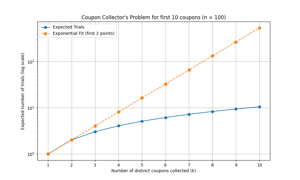
It’s a poor fit. The exponentially increasing difficulty of finding a new species is not well-explained by the coupon collector’s problem, the power-law distribution must be the real reason. But that just poses a new question: why are the probabilities of species power-law distributed?

Here’s another question: why aren’t coverage-guided fuzzers asymptotically better than this? Indeed, at the Antithesis conference, Zac Hatfield-Dodds suggested that they are. He gave a talk about his property-based testing library Hypothesis, and threw out a thought-provoking aside. If I heard him correctly, he said “coverage-guided fuzzing reduces the time to find a bug from exponential to polynomial.” This paper seems to contradict him, but perhaps I don’t understand his meaning. I need to think or investigate more.

Nondeterministic Programs

Now things get really hard. Multithreaded programs interleave instructions nondeterministically, and distributed systems suffer unpredictable network delays, message loss, and clock skew. When you test these programs, not only must you try lots of inputs, but you must try each input many times.

If you run the same test of a nondeterministic program repeatedly, you’ll probably get different outcomes, but not efficiently: mostly the program will just follow the same path over and over without discovering new bugs. You can explicitly increase randomness by introducing random network delays or various faults, as Jepsen does.

You can find concurrency bugs in multithreaded programs much more efficiently if you control thread scheduling. Finn Hackett, a MongoDB PhD fellow and intern, showed me the paper A Randomized Scheduler with Probabilistic Guarantees of Finding Bugs, in ASPLOS 2010. The authors point out that even a simple multithreaded program has an overwhelming number of possible schedules: n threads that collectively execute k instructions have on the order of n^k schedules. But only some of the scheduling choices matter for reproducing any of the program’s concurrency bugs. This paper defines a nice term, bug depth, “the minimum number of scheduling constraints that are sufficient to find a bug.”

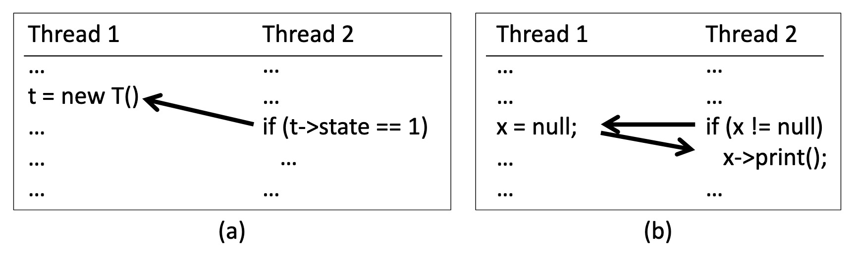
For example, in the paper’s Figure 1(a), a bug is reproduced if Thread 2 accesses a variable before Thread 1 initializes it. This bug has one scheduling constraint, i.e. depth 1. In Figure 1(b), the bug requires Thread 1 to run an assignment after Thread 2 runs an if-statement and before it runs a method-call, so it has depth 2. The authors describe a thread-scheduling algorithm that finds any single bug of depth d with probability 1/nk^d-1, much better than the theoretical lower bound of 1/n^k, i.e. the probability of picking one schedule out of all possible schedules. You can expect to find a depth-1 bug in an n-threaded program in n tries and a depth-2 bug in nk tries.

Their algorithm is called Probabilistic Concurrency Testing (PCT). You provide PCT with a program that executes up to k instructions on n threads. You provide a desired bug depth d, and an input that could trigger a bug of depth d. PCT’s job is to find a schedule that does trigger it. PCT assigns random initial priorities d, d+1, …, d+n to the n threads. PCT chooses d-1 random “change points” in the program. It allows the program to execute one instruction at a time on one thread: the highest-priority runnable thread, i.e. the thread with the largest priority number that isn’t waiting for anything. When a thread stumbles upon the i^th change point, PCT changes the thread’s priority to i and continues. PCT uses higher numbers for threads' initial priorities (≥d) than it uses for change points (<d), so that a thread tends to be unscheduled when it hits its first change point, perturbing the system and increasing the chance of bugs.

Here’s Figure 6(b) from the paper. It shows the same depth-2 bug as before. PCT reproduces it by assigning priority 3 to Thread 2, and priority 2 to Thread 1 (white circles), and inserting a change point (black circle) that changes Thread 2’s priority to 1. The probability of PCT assigning these initial priorities is 1/n, and its probability of choosing this change point is 1/k. Thus there’s a 1/nk chance of finding this bug in one try, which matches the authors' promise of finding a depth 2 bug in nk tries on average.

In practice PCT is much more efficient than its worst-case bound, since there are usually many ways to reproduce a given bug.

The authors implemented PCT for real:

For fine-grained priority control, we implemented PCT as a user-mode scheduler. PCT works on unmodified x86 binaries. It employs binary instrumentation to insert calls to the scheduler after every instruction that accesses shared memory or makes a system call. The scheduler gains control of a thread the first time the thread calls into the scheduler. From there on, the scheduler ensures that the thread makes progress only when all threads with higher priorities are blocked.

I think by “shared memory” they mean the heap, which is shared among threads. In the abstract description above we called the total number of instructions k, but the authors' implementation of PCT only places change points before synchronization points, like pthread calls or atomics, and k is the number of these synchronization points. Surprisingly, PCT can run huge programs like Mozilla at one-third normal speed. The paper’s evaluation section describes the bugs they found and how quickly, and the various optimizations and heuristics they added to the algorithm. This part interested me:

Final Wait: Some concurrency bugs might manifest much later than when they occur. We found that PCT missed some of the manifestations as the main thread exits prematurely at the end of the program. Thus, we artificially insert a priority change point for the main thread before it exits.

There must be hordes of rarely-manifesting use-after-free bugs where the main thread deletes global variables as it exits, and background threads sometimes wake up just before the program terminates.

Deterministic Simulation Testing

At MongoDB we run certain concurrency tests, which we know are highly nondeterministic, many times each night. There are rare bugs that pop up once every few months, or few years. This is bad, because we don’t know which change introduced the bug, and once we diagnose it, we can’t be confident we fixed it.

Some companies like FoundationDB built deterministic simulation testing into their code from the start. When FoundationDB was acquired by Apple, some of the FoundationDB team left to create Antithesis and bring deterministic testing to projects that didn’t build it in. Running MongoDB’s nondeterministic tests in Antithesis has been helpful, and I expect we’ll use them more.

Inconclusion

Distributed systems engineers (myself included) typically aren’t knowledgeable enough about randomized testing and we don’t deploy it thoughtfully. We should ask rigorously, exactly how much confidence do I gain with each trial, and how can I test nondeterministic programs efficiently? And the most vexing question of all: when can I stop? I don’t know the answers yet.

Images: Fabre’s Book of Insects (1921)