Paper review: Scaling Large Production Clusters with Partitioned Synchronization
Scaling Large Production Clusters with Partitioned Synchronization, USENIX ATC 2021. One of the “best paper” award winners.
In this paper, researchers from Alibaba and Chinese University of Hong Kong design a distributed task scheduler. They have a cluster with thousands of worker machines, and the task scheduler’s job is to choose a “resource slot” on one of these machines for each new task to use. Alibaba’s prior system used a single scheduler, which conked out at a few thousand new tasks per second. They want to design a distributed task scheduler that can scale to 40K new tasks per second, backed by 100k worker machines. They find that just adding more schedulers or more resources yields diminishing returns, so they seek other optimizations. They find that when multiple schedulers are running at once, the staleness of each scheduler’s view of the global state contributes to scheduling conflicts, which slows down the system. To reduce maximum staleness they design Partitioned Synchronization, and they describe how to balance high-quality versus low-latency scheduling.
Table Of Contents
System Model #
The action begins when a client submits a task to a scheduler. The scheduler chooses a “resource slot” to commit to the task. The task runs using the slot until the task finishes. Tasks run for 5 seconds on average; most seem to range between 1 and 10 seconds.
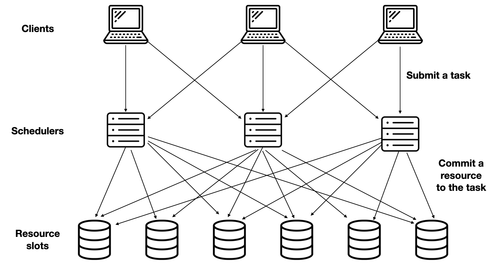
The authors don’t describe what they mean by a “slot”; I assume it’s a slice of one machine’s resources. Each slot can be committed to only task at a time. Not all slots are the same: some have more CPU, or more RAM, or they are closer or farther to the data needed by a certain task, or they have certain previous tasks’ data cached.
Their goals:
- A distributed task scheduler that can handle about 40k new tasks/sec.
- Low-latency, high-quality scheduling.
Low latency means a task is quickly assigned to a machine and starts executing. High quality means a task is assigned to a suitable machine, and that global measurements like fairness are close to ideal. Quality isn’t defined in detail here, which I think is the paper’s greatest weakness. I’ll say more below.
Their constraints:
- Can’t statically partition resources among schedulers.
- Can’t have single master scheduler.
They can’t just divide the number of machines by the number of schedulers and give each scheduler exclusive access to a subset of machines. They say this leads to under-utilization if some partitions are more idle than others, and there are global properties they want to uphold that require schedulers to be aware of the whole state, not a subset. They can’t have just one scheduler because it can’t assign tasks fast enough, it has to be scaled out.
Baseline Scheduler #
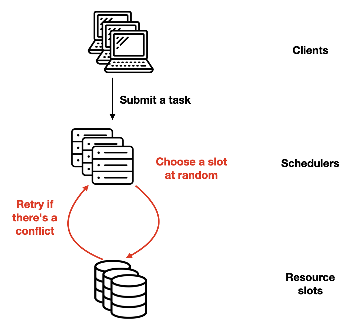
The authors describe the simplest possible scheduler algorithm, for the sake of analysis. Each scheduler just assigns each task at random to some slot. There’s no attempt to maximize quality. Often, multiple schedulers assign different tasks to the same resource: this is a “scheduling conflict.” One succeeds and the rest of them retry, which adds latency.
What’s the cost of conflicts, and how can we reduce them? Let’s say each scheduler can handle K tasks per unit of time if there are zero conflicts. So, if there are J new tasks per unit of time, we need N = J / K schedulers. But there will be conflicts, since schedulers just choose slots at random. If S slots are exactly enough to execute all the tasks, let’s add Sidle additional slots to reduce conflicts.
The authors do a half-page of math to derive the expected number of conflicts per unit of time: 
- N : number of schedulers
- K : tasks per second
- Sidle : additional slots
This formula’s main message is more slots are better. If you graph it with some arbitrary constants for N and K, you see it’s asymptotically decreasing:
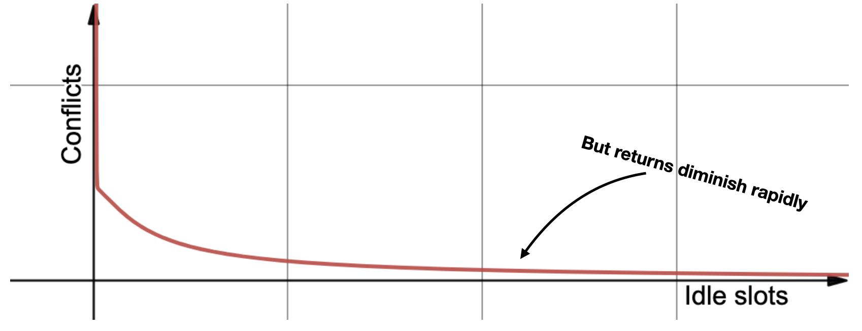
So, the more idle slots you have, the fewer conflicts, thus fewer retries, thus less scheduling latency. But there’s diminishing returns. Remember, idle slots are expensive computers in a hot data center, and you’re not even using them!
The authors apply the same argument to schedulers, and find diminishing returns again: More schedulers reduce latency by spreading the load, but they also conflict with each other more and cause more retries.
A More Realistic Simulation #
The previous formula is simplistic, so the authors want to simulate their system with more realism. They add two variables:
- G : The synchronization gap.
- V : The variance of slots’ scores.
Each scheduler has its own view of the global state, i.e., which slots are committed and which are idle. A slot’s state changes when another scheduler commits it to a task, or when a task finishes, but there’s a “synchronization gap” G between these changes and the moment when the scheduler learns of them by periodically refreshing. The less frequent these refreshes, the staler the scheduler’s view on average, which means more scheduling conflicts.
In the authors’ simulation, each slot has a single “score” which determines how fast it runs tasks. The variance of scores is V. I think this is a misstep. As the authors note, different tasks have different needs. A slot’s score is in the eye of the beholder. In reality, a slot’s score is a function of the slot and the task, and a good scheduler should commit a slot to the task that wants it more than other tasks want it. I believe this oversimplification in the simulation means they actually underestimate how good their solution is.
Partitioned Synchronization #
We saw above that adding idle slots and adding schedulers is an expensive way to reduce scheduling latency. The authors try two new tactics:
- Reduce the staleness of schedulers’ local states.
- Sacrifice scheduling quality when necessary to reduce scheduling latency.
Their solution is called Partitioned Synchronization, or ParSync. In this system, they divide the resource slots evenly into P partitions. (It seems like P must be divisible by N, the number of schedulers. If it were me I’d just set P = N, but maybe there’s some reason more partitions useful.) Instead of synchronizing all schedulers’ state every G seconds, the system refreshes each scheduler’s view of different partitions in each synchronization round. Therefore a sync round is shorter, it takes only G / N seconds. The partitions are reassigned round-robin, so after N rounds all schedulers have synced all partitions and the cycle repeats.
Note that each scheduler has a fresher view of its most recently synced partition than all other schedulers do. This will be important later.
Total Staleness #
The authors said their goal was to reduce staleness, but they achieve something subtler: although average staleness is the same as before partitioning, the variance of staleness is smaller.
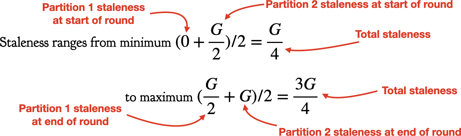
Without partitions, each scheduler’s view of the slots’ state is refreshed every G seconds. All schedulers’ staleness ranges from 0 to G, and the average is G / 2.
But with two partitions, each sync round takes G / 2 seconds and refreshes half the partitions. Let’s consider one of the schedulers in the fleet. At the beginning of some round, its view of Partition 1 has 0 staleness (it was just refreshed) and its view of Partition 2 has G / 2 staleness (it hasn’t been refreshed since the previous round). At the end of this round the Partition 1 staleness has grown to G / 2, and the Partition 2 staleness to G. Then the scheduler refreshes Partition 2 and the cycle repeats, with the partitions’ places swapped.
Average total staleness is always G / 2. But the range of staleness is smaller with two partitions. Instead of ranging from 0 to G, it ranges from G / 4 to 3G / 4. With more partitions the range is even smaller.
The authors write:
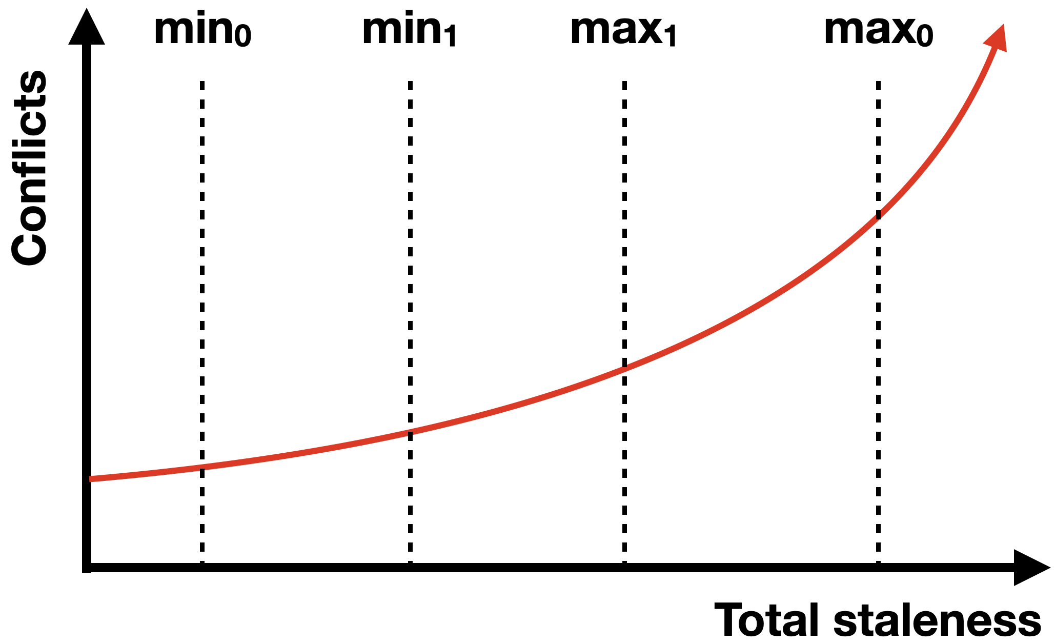
Scheduling delay increases disproportionately within the period G. When the cluster state is just synchronized, it is fresher and scheduling has fewer conflicts. But when the state becomes more outdated towards the end of G, scheduling decisions result in more conflicts. Conflicts lead to rescheduling, which may in turn cause new conflicts, and hence rescheduling recursively.
A smaller maximum staleness saves more conflicts than a larger minimum adds. Consider the area under the curve between min0 and max0. If you narrow the lines to min1 and max1, you delete more area from the right than you add on the left.
Quality vs. Scheduling Latency #
After each partitioned synchronization round, each scheduler has a fresh view of some partitions and a stale view of others. A scheduler can minimize conflicts (and therefore latency) by committing slots from its freshest partitions, or it can maximize quality by committing the best slots first, regardless of which partitions they’re in. So the authors identify three scheduling strategies:
- Latency-first: Look for high-quality slots in the freshest partitions first.
- Quality-first: “First choosing the partition with the highest average slot score and then picking available slots by weighted sampling based on slot scores.” (Why so complicated? To reduce conflicts from all schedulers rushing for the top-scoring slots?)
- Adaptive: Use Quality-first, but if latency exceeds some SLA switch to Latency-first.
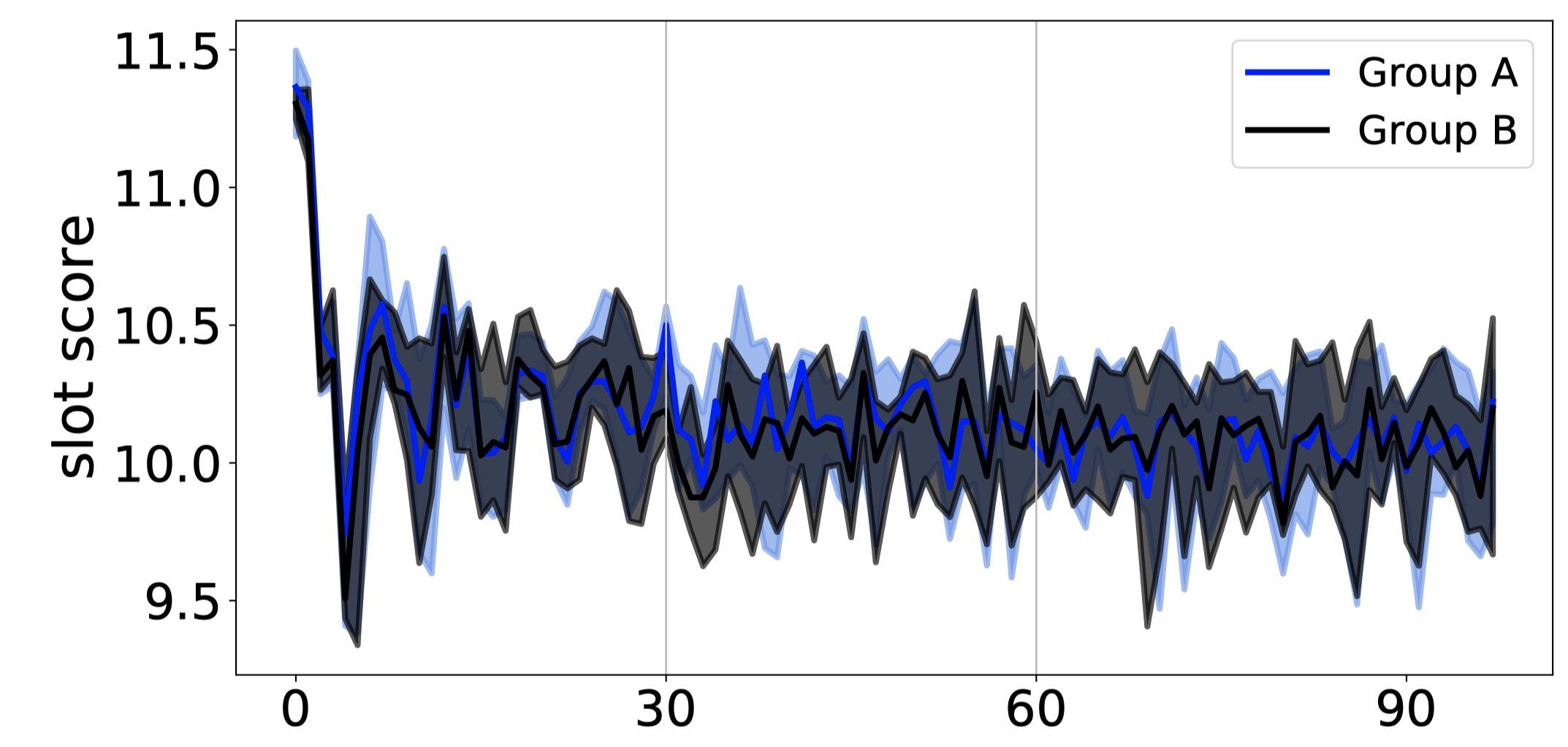
They simulate an experiment with a cluster of 200k slots. Each task takes exactly 5 seconds and requires 1 slot. There are two scheduler groups. The simulation has three phases:
- 0-30 seconds: low load.
- 30-60 seconds: high load on scheduler group A.
- 60-90 seconds: high load on scheduler groups A and B.
Already I have some criticisms:
- Wait, what’s a “scheduler group”? This is an unexplained swerve. Why would one group have higher load than the other? Shouldn’t clients submit tasks to all schedulers evenly?
- Since real tasks have varied duration, I think it would be more realistic to vary the simulated tasks’ durations.
- As I said above, giving each slot a single “score” ignores that some tasks prefer different slots than other tasks.
- What’s the point of “score” if a higher-scoring slot doesn’t execute a task in less time?
The following charts are the authors'.
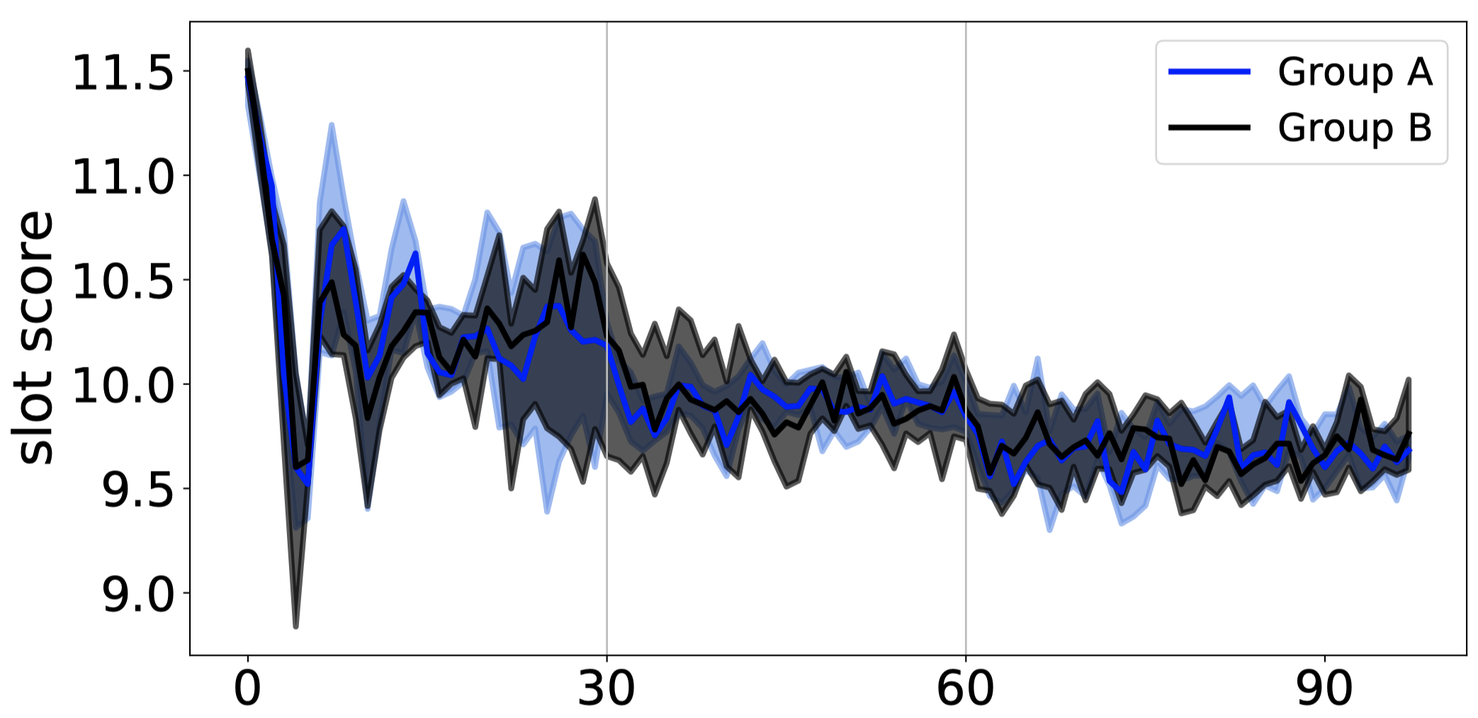
Quality-first: Quality
The Quality-first scheduler mostly picks the slots with the highest scores first, so its average score starts high, then drops as the high-quality slots are used up. To my eye there’s some regular oscillation amid the noise, perhaps this is the periodic refresh (after each refresh, schedulers all rush to use the high-quality slots that were freed since the last refresh), or perhaps it’s because the tasks all take exactly 5 seconds.
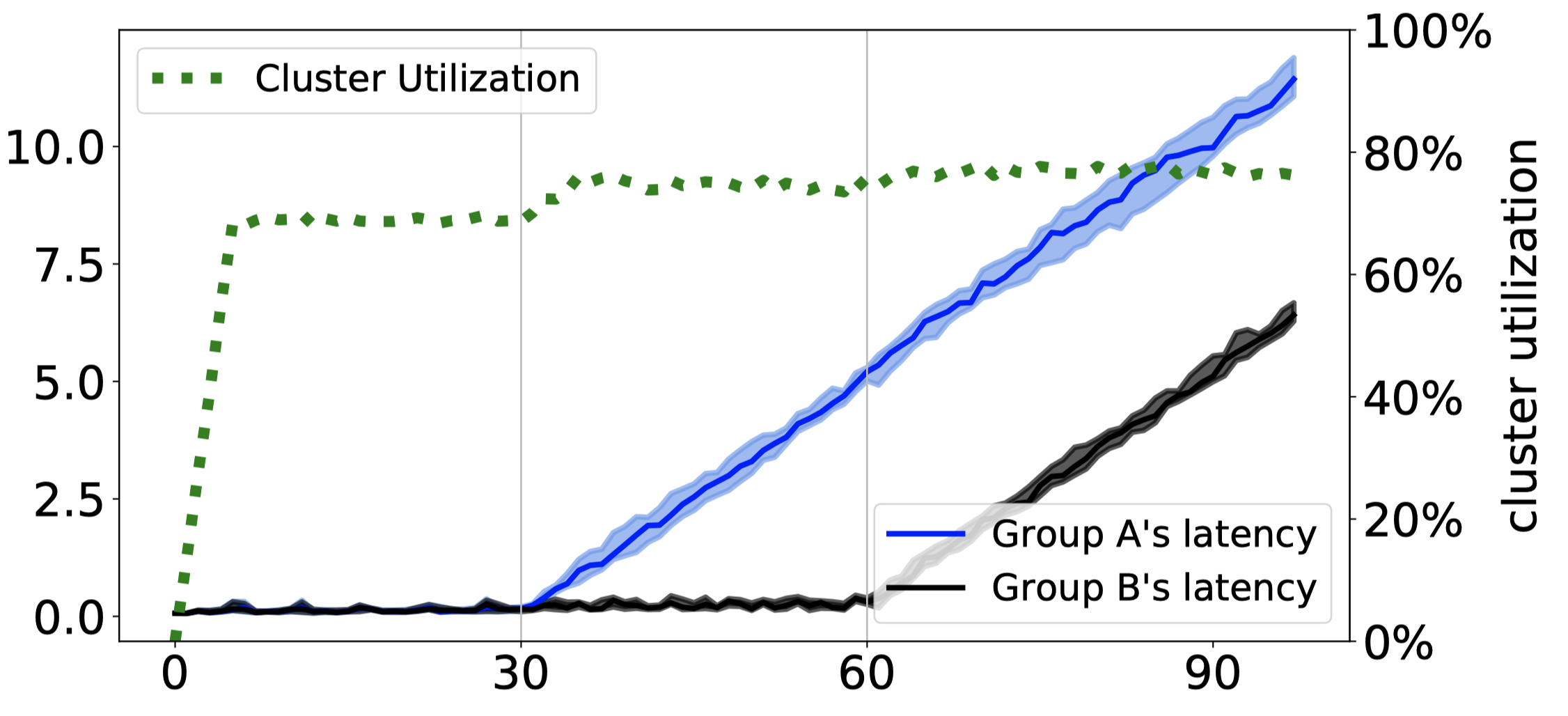
Quality-first: Delay
Since, for some reason, schedulers in Group A get pummeled for 30 seconds while Group B is underutilized, it’s no surprise that Group A begins to fall behind first. As soon as a scheduler group is overloaded, its queues grow at a constant rate and latency increases linearly, forever. The Quality-first strategy has no solution to this.
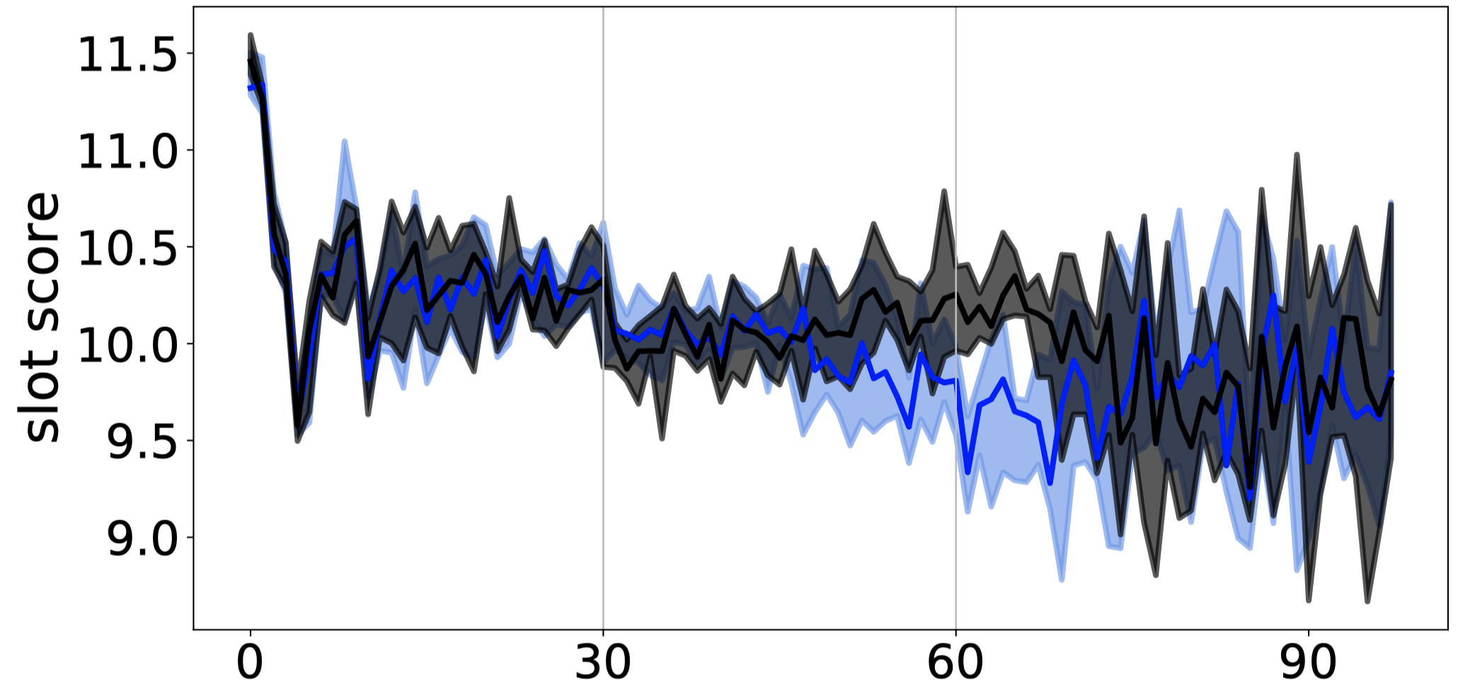
Latency-first: Quality
The Latency-first scheduler still prefers high-score slots (in each scheduler’s freshest partitions) so quality begins high and starts oscillating. Interestingly, the average score is almost as good as Quality-first, and the variance is smaller. Whether the slightly worse quality matters depends on what “quality” is measuring in some real system.
However, the author’s simplistic simulation of quality hurts the Quality-first strategy. If Sidle = 0 then I think there’s no point at all to the Quality-first strategy: Since all tasks value high-score slots equally, all the schedulers rush to grab the high-score slots first, and then they all have to fall back to lower-score slots, until all the slots are used. What order the slots are chosen barely affects the overall quality score, as we see in the charts.
But in real life, certain tasks really benefit from using certain resources. A Quality-first scheduler could achieve a higher overall quality score by carefully matching tasks to the slots they prefer, the same as international trade raises global productivity via comparative advantages. Plus, in real life tasks finish faster when they have the slots they prefer, which frees slots faster, and thus reduces latency and improves the quality of future scheduling rounds.
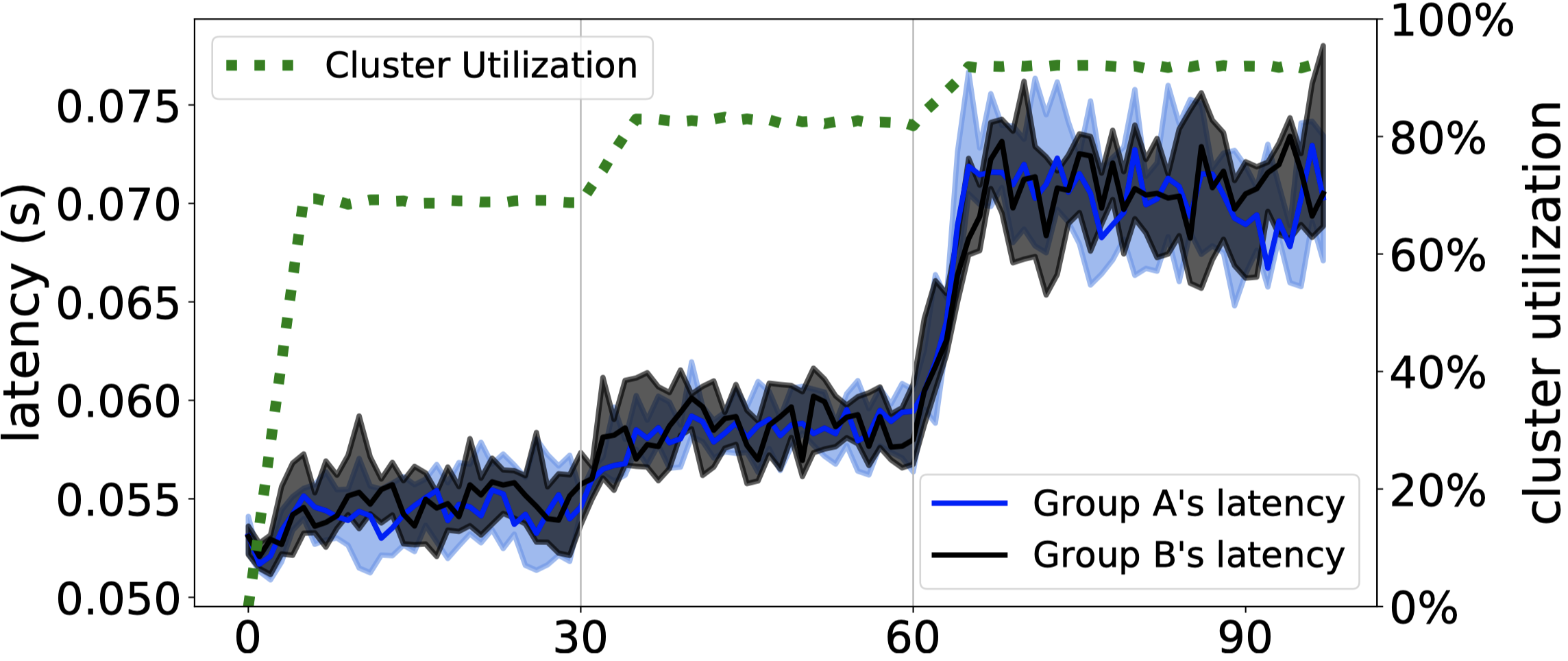
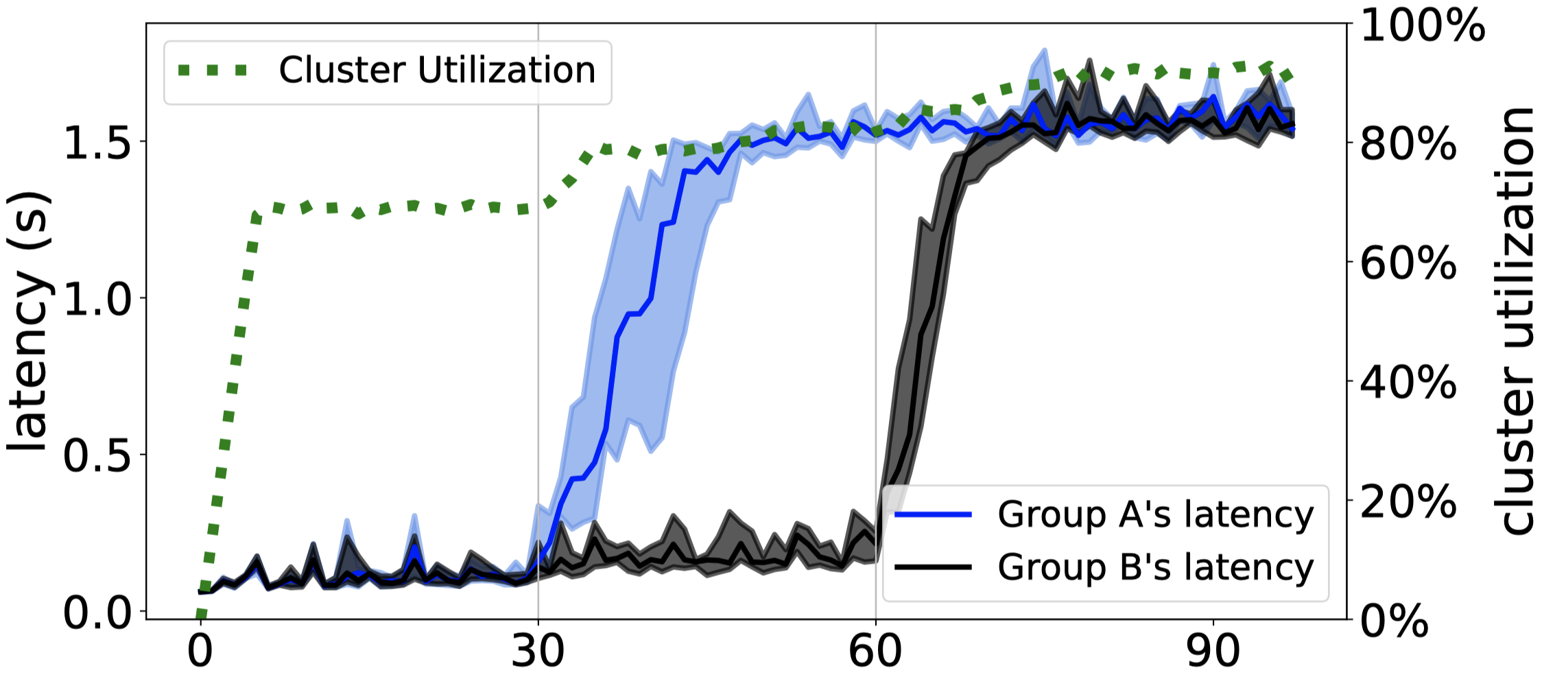
Latency-first: Delay
I don’t understand this chart. Groups A and B must be cooperating somehow, since their latencies both rise a little when Group A is overloaded, then both rise a lot once Group B is also overloaded. The interactions between the groups aren’t explained in the paper. Anyway, notice that this chart’s latency axis is very different from the axis on the Quality-first chart: its latency is capped near 0.75 seconds, versus Quality-first’s 10 seconds and infinitely rising. 1.5 sec is the chosen SLA
Adaptive: Quality
The Adaptive strategy uses Quality-first until latency exceeds a chosen SLA (1.5 seconds in this simulation), then switches to Latency-first. Since quality is not realistically simulated, all the strategies appear to have similar quality. It’s surprising the quality variance increases after the strategy switches to Latency-first (since above we saw the Latency-first has smaller variance), but I wouldn’t put too much stock in these quality charts anyway.
Adaptive: Delay
The system works as designed: it lets latency rise to 1.5 seconds, then caps it.
Their Evaluation #
The authors say that partitioned synchronization “increases the scheduling capacity of our production cluster from a few thousand tasks per second on thousands of machines to 40K tasks/sec on 100K machines…. ParSync effectively reduces conflicts in contending resources to achieve low scheduling delay and high scheduling quality.” The Adaptive scheduling strategy balances quality and scheduling latency.
My Evaluation #
The ParSync algorithm is very clever, and nicely explained. I bet a whole class of distributed task schedulers can benefit from it.
The paper could’ve spent less time analyzing non-ParSync algorithms; the main action doesn’t start until late in the show.
Their simulation is marred by their simplistic assumptions that all tasks prefer the same slots (measured by a single “score” for each slot), and that all tasks take exactly 5 seconds to run, regardless of which task is running or which slot it uses. This underrates the value of “Quality-first” scheduling. It may underrate the value of the authors’ entire contribution. I wish they had used a better simulation, so I could fully appreciate ParSync.
This paper is a good followup to Protean: VM Allocation Service at Scale.
See also: