Paper Review: E-Store, P-Store, and Elastic Database Systems
Elastic Database Systems, a 2017 PhD thesis by Rebecca Taft, collects several techniques for auto-scaling a sharded database. Each technique is so direct, so obviously useful, that I can hardly believe I didn’t encounter it earlier: a sure sign of a really good new idea. This research is even more relevant today, when companies selling serverless databases must compete on efficiency.
I’ve read Taft’s thesis, plus two papers that summarize the same material:
- E-store: Fine Grained Elastic Partitioning For Distributed Transaction Processing Systems, VLDB 2015.
- P-Store: An Elastic Database System with Predictive Provisioning, SIGMOD 2018.
Taft is the lead author on both; famous researchers Michael Stonebraker and Andy Pavlo are among the coauthors. If my summary gets you excited, I recommend you read the thesis rather than the papers. The papers are very dense to meet conferences’ demand for unreasonable concision. The thesis has more pages, but it’s less total effort to comprehend.
Taft’s research prototypes are built atop H-Store, a research prototype database. It’s in-memory and sharded. (It could be replicated too, but Taft ignores replication for simplicity.) H-Store is a very cool project in its own right, you can read papers about it or its commercial variant, VoltDB.
Taft’s thesis describes two systems, E-Store and P-Store. The first is reactive: like most autoscaling systems I’ve read about, it measures load and scales in/out in reaction to rising/falling demand. What makes it clever is how it quickly smooths out uneven load. P-Store, on the other hand, is predictive: it forecasts demand based on past cycles and starts scaling in/out at the right time to minimize cost. In both cases, the goal is to build an auto-scaling distributed data store on top of a virtual machine provider like EC2, paying the provider as little as possible while always meeting the demands of a fluctuating workload. I found P-Store revelatory so I’ll spend most of our time there.
E-Store #
E-Store is designed for a sharded database with a skewed workload; i.e., some tuples are hotter than others. (A “tuple” is also known as a record, row, document….) Like most sharded databases, E-Store partitions its data into disjoint blocks. Each block contains tuples within some key range. Each machine stores many blocks. If a block contains some hot tuples, its machine risks overload. But now the system faces a Catch-22: moving a whole block of data from an overloaded machine will temporarily make the overload worse, and it will take a long time. So E-Store identifies individual hot tuples and tracks them separately, so it can quickly move one hot tuple from an overloaded machine. This is fast and cheap and relieves the hot spot right away. Later if the hot tuple becomes cold, E-Store merges it back into its block and stops tracking it separately.
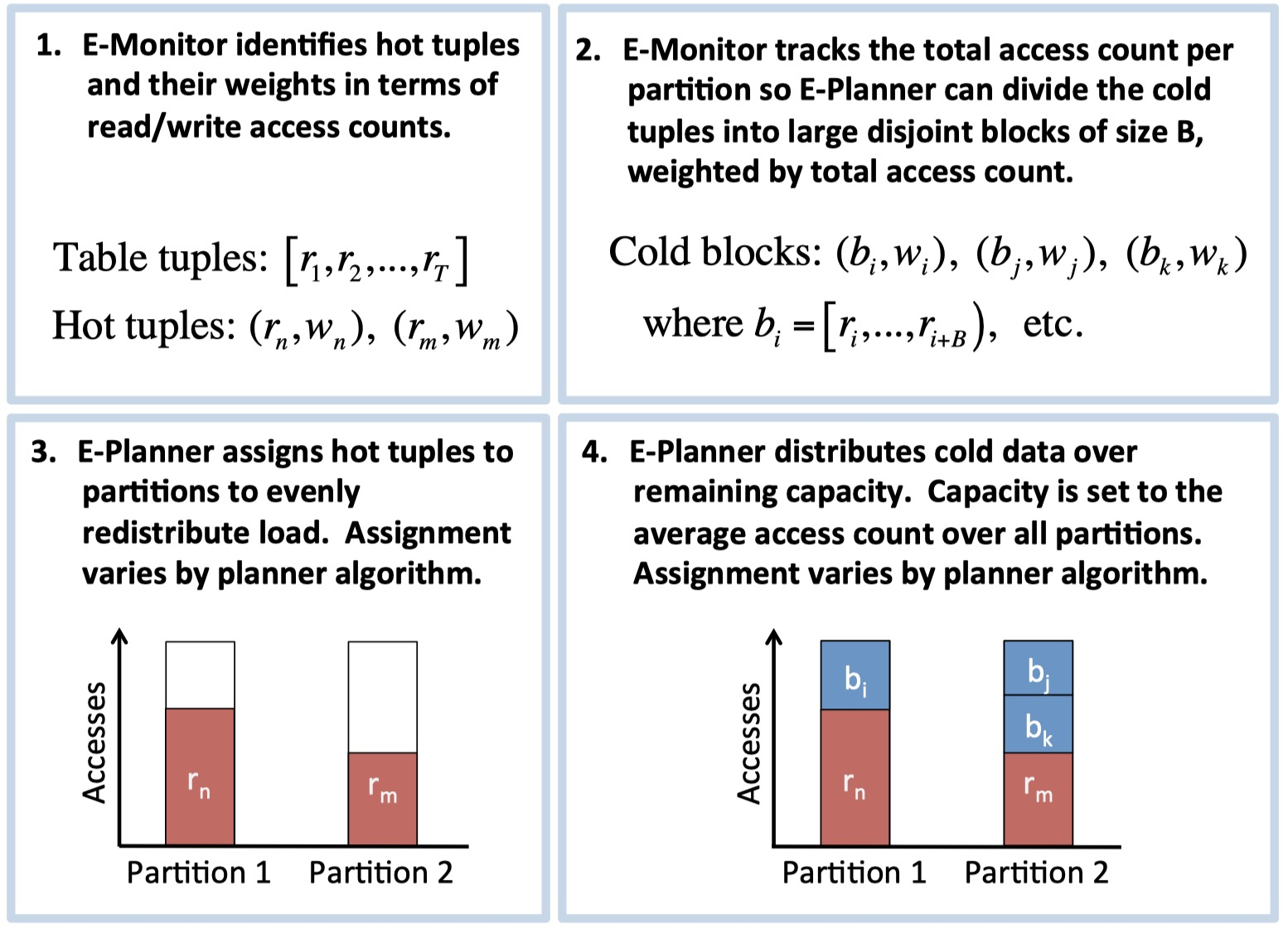
Steps of E-Store's migration process. Credit: Taft et al.
Taft describes several optimizations that make E-Store more sophisticated than most autoscaling systems I’ve read about. It uses cheap CPU monitoring most of the time; only when it detects an imbalance does it switch briefly to expensive per-tuple monitoring. The rebalancer chooses a plan that minimizes data movement while achieving a reasonably balanced outcome. It prioritizes moving hot tuples rather than cold blocks. As a result, E-Store can handle spikey and skewed workloads with fewer latency spikes than comparable systems.
P-Store #
The insight that motivates P-Store is that many workloads are cyclic, and therefore predictable. The authors used historical data from a Brazilian retailer called B2W, known as “the Amazon of Brazil”. (I thought the Amazon of Brazil was a river, but no, we live in an absurd era, nothing is real.) B2W’s load is spikey—its peak is 10x its trough—and cyclical: it has daily and weekly cycles. (And yearly, although the authors don’t handle that.)
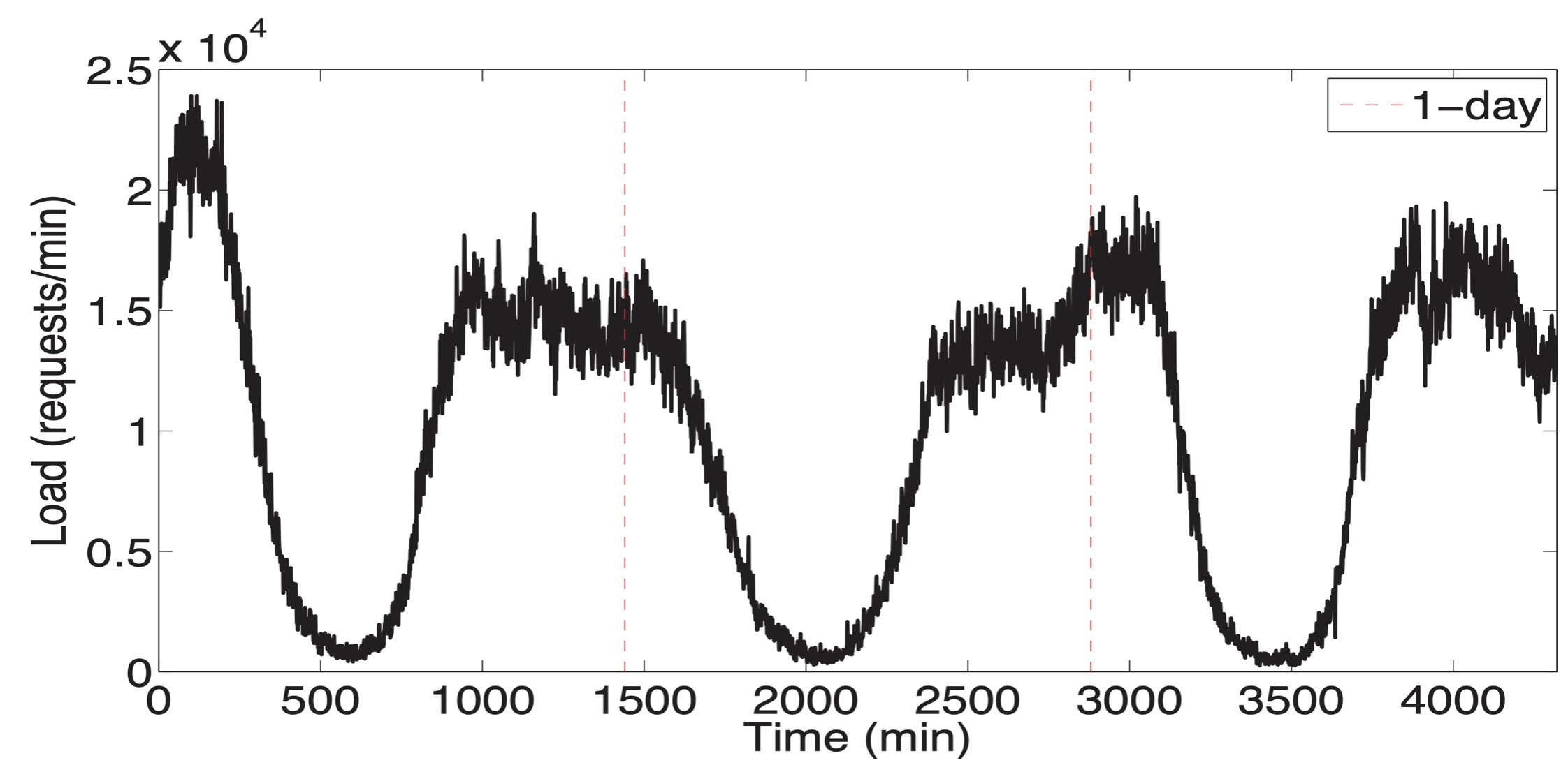
Load on one of B2W’s databases over three days. Credit: Taft et al.
When a reactive system deals with fluctuating demand like this, it scales out while load is spiking. Thus it faces a tradeoff: it must either pay for lots of spare capacity during stable periods, or suffer bad performance while it scales out during the spike. P-Store finds a better way. It analyzes past cycles to forecast future changes in demand, so it starts scaling out before a spike. It also forecasts how long scale-out will take, so it can start at the right time. This prescience lets P-Store minimize overhead without risking bad performance.
Modeling the system #
P-Store has to know the system’s capacity per server and how quickly it scales in/out, so P-Store can decide when to start scaling in anticipation of a change in demand. It models the system with three variables:
- Q̂: The max capacity of one server. The authors determine this experimentally by loading a server until latency rises, then reducing to 80% of that load for safety.
- Q: The target throughput, how much load P-Store aims for each server to experience in a stable, balanced system. Set to 65% of Q̂ to leave headroom for the costs of the scaling process.
- D: The data-transfer speed during rebalancing. The authors determine this experimentally, too, by transferring data faster and faster between servers experiencing Q̂ of regular load, until the data transfer affects the latency of normal operations. Then they set D to 90% of this speed for safety.
You can see there’s still lots of headroom built in to deal with unforecasted spikes, skewed workload, etc. I’m curious how the authors decided the amount of buffer needed, and whether a real world system with experienced operators could run closer to the maxima.
Forecasting demand #
P-Store uses Sparse Periodic Auto-Regression (SPAR) to find cycles in the past week of history. It also measures an offset between the last 30 minutes of load and the average for that time of day and day of week. This offset might indicate long-term growth or decline, or some unusual event taking place. P-Store combines the offset with the periodic prediction to forecast the next 60 minutes of demand.
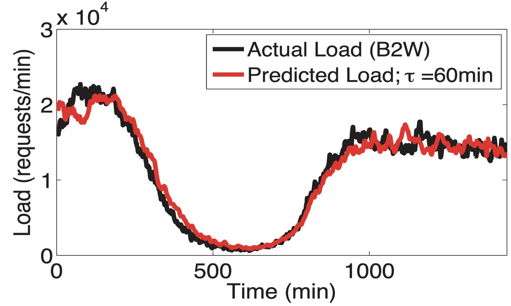
60-minute-ahead SPAR predictions during a 24-hour period. Credit: Taft et al.
You can see that SPAR with these parameters predicts B2W’s workload very accurately, with relative error around 10%.
Effective capacity over time #
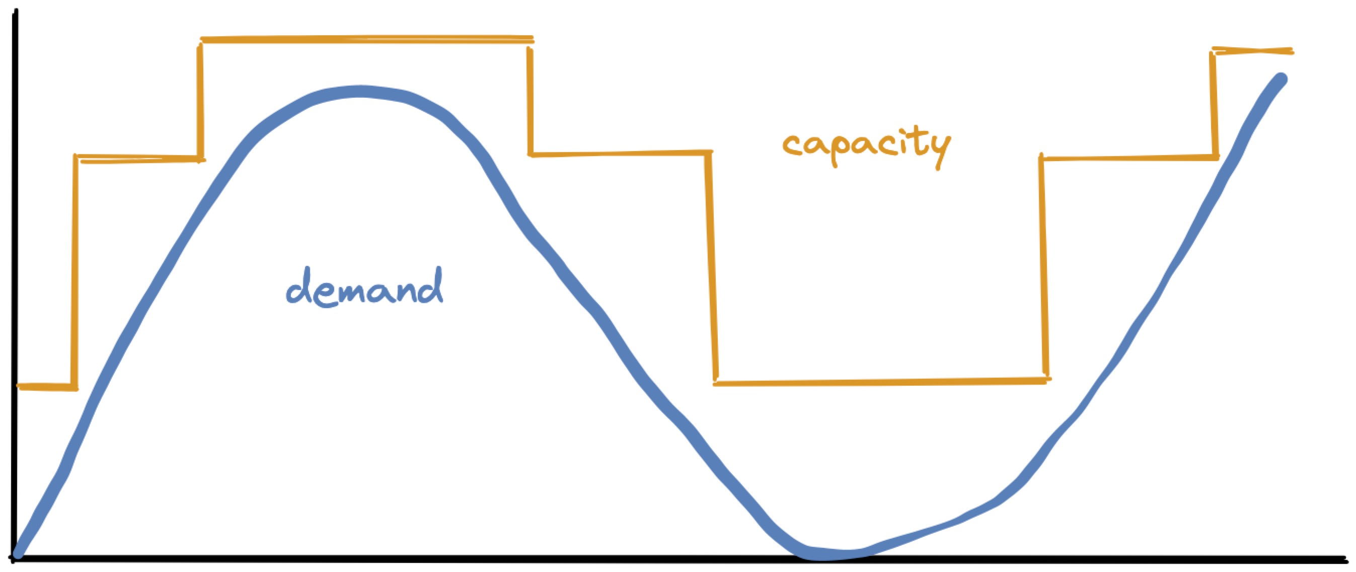
Given a prediction about how workload will fluctuate, P-Store must decide when to add or remove machines, and how many. Its goal is to match the forecasted demand (blue) with capacity (orange), with just a little headroom for safety:
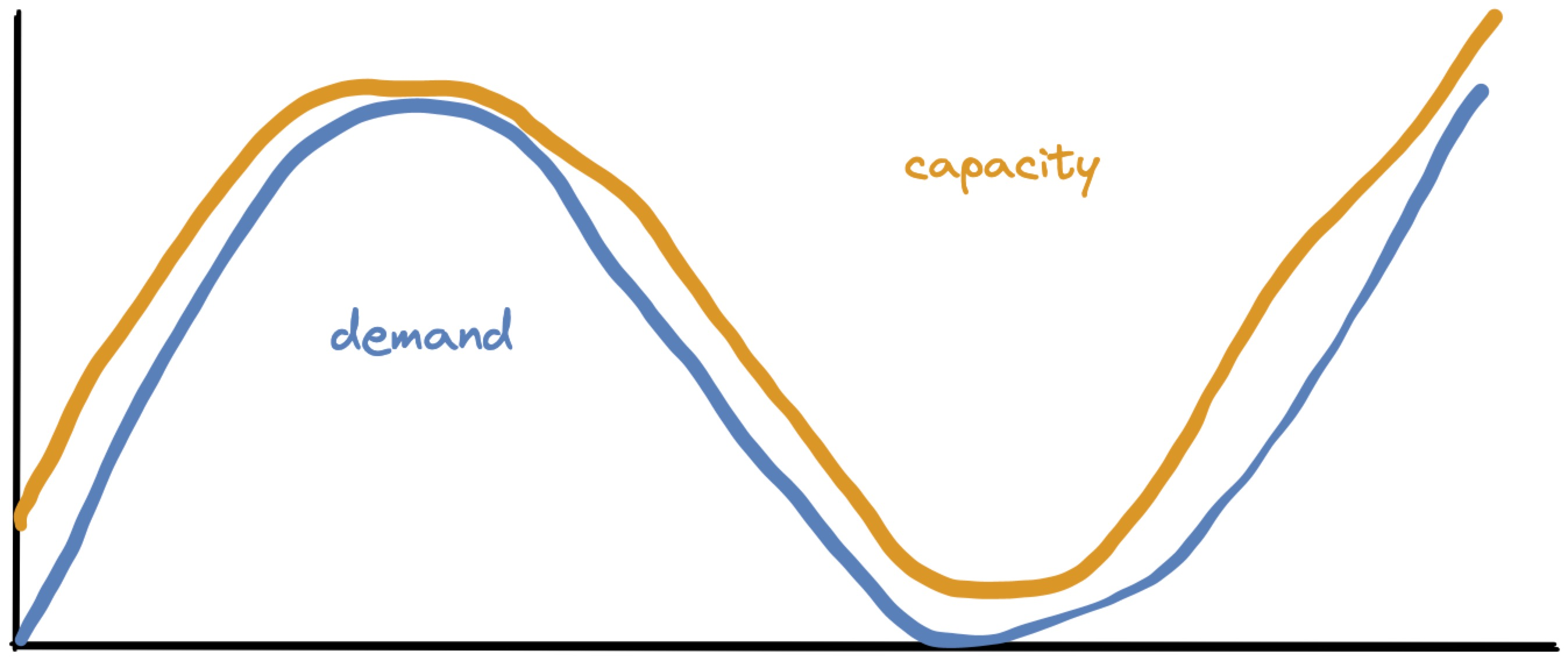
But P-Store can’t continuously vary capacity. It adds and removes whole machines, so capacity is a step function:
There’s one more complication. When P-Store adds a machine, the system’s capacity doesn’t jump upward immediately. What Taft calls “effective capacity” curves upward over time, as chunks of data are migrated onto the new machine, until the data is fully balanced:
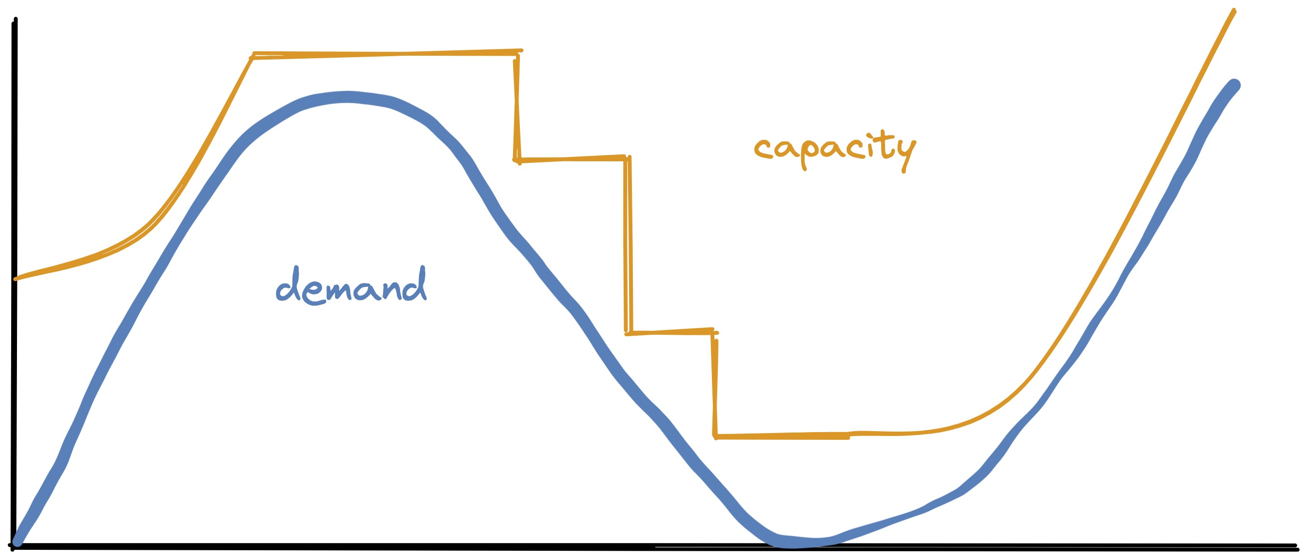
(When a machine is removed, I’m showing effective capacity drop instantly. I’m not sure this is how it works in the real world or P-Store’s model.)
Planning to meet demand #
P-Store evaluates its current situation and plans for the immediate future. It looks at a week of history leading up to the current moment, and uses it to forecast the next hour. Then it decides what steps it should take for the next hour to match demand. Finally, it executes the next single step: it scales out or in by some amount, or maintains the status quo.
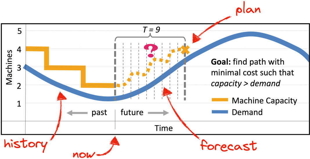
The planner's goal. Credit: Taft et al. I added the red arrows.
Note, even if demand is currently steady or falling, P-Store might need to start scaling out now to meet demand that will come within the next hour. This is why P-Store forecasts and plans far ahead, although each step requires just a few minutes to execute, and P-Store reevaluates every few minutes.
So how does P-Store decide what to do?
In order to determine the optimal series of moves, we have formulated the problem as a dynamic program. This problem is a good candidate for dynamic programming because it carries optimal substructure. The minimum cost of a series of moves ending with A machines at time t is equal to the minimum cost of a series of moves ending with B machines at time t − T(B,A), plus the (minimal) cost of the last optimal move, C(B,A).
Taft describes the algorithm in a couple pages of pseudocode. Here’s my understanding.
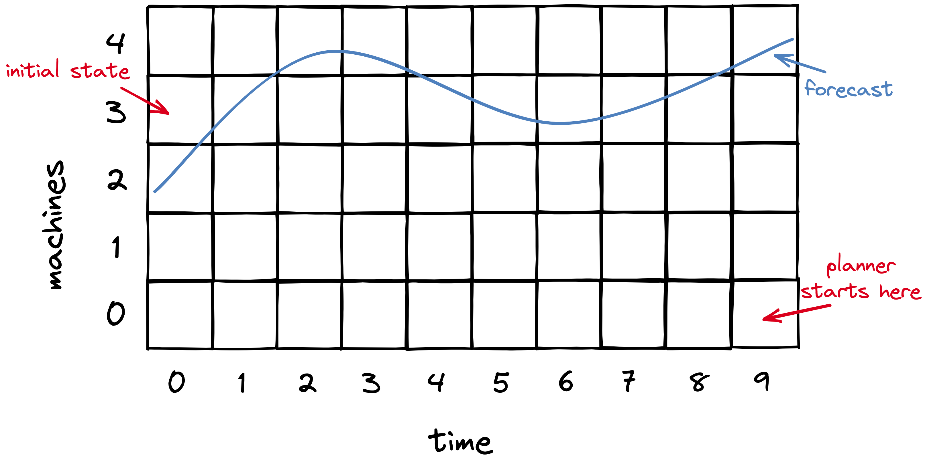
The planner’s main data structure is a matrix. Each column is a time slot in the future; the planner decides what step it will take at each of these times. Each row is a number of machines that might be allocated, up to a maximum determined by the max load forecasted. In each cell, the planner will memoize the cost of the cheapest “feasible” path to that cell. A path is feasible if there are enough servers to handle forecasted load at each step from the initial cell to the destination cell. I imagine (and this is my invention) that you could draw the forecasted load superimposed on the matrix (blue line) to visualize feasible paths.
The planner begins on the lower right: this is the cheapest possible end-state. However, there’s no feasible path to it, since there aren’t enough machines at that end-state to handle load. The planner considers an infeasible path to have infinite cost, and since all paths to the lower-right cell are infeasible, the cell’s cost is infinite.
The planner proceeds to consider each end-state cell, from bottom to top, i.e. from the least number of machines to the most. The next few cells have infinite cost, but finally we reach the 4-machine row, which is the first with a feasible path to it. The planner does a depth-first search of paths from the initial state to this end-state, calculating each path’s cost as the sum of the number of machines allocated in each time slot. It recursively selects the cheapest path leading to each cell from left to right. It never has to recalculate the cheapest path to a given cell because it memoizes that info in the matrix.
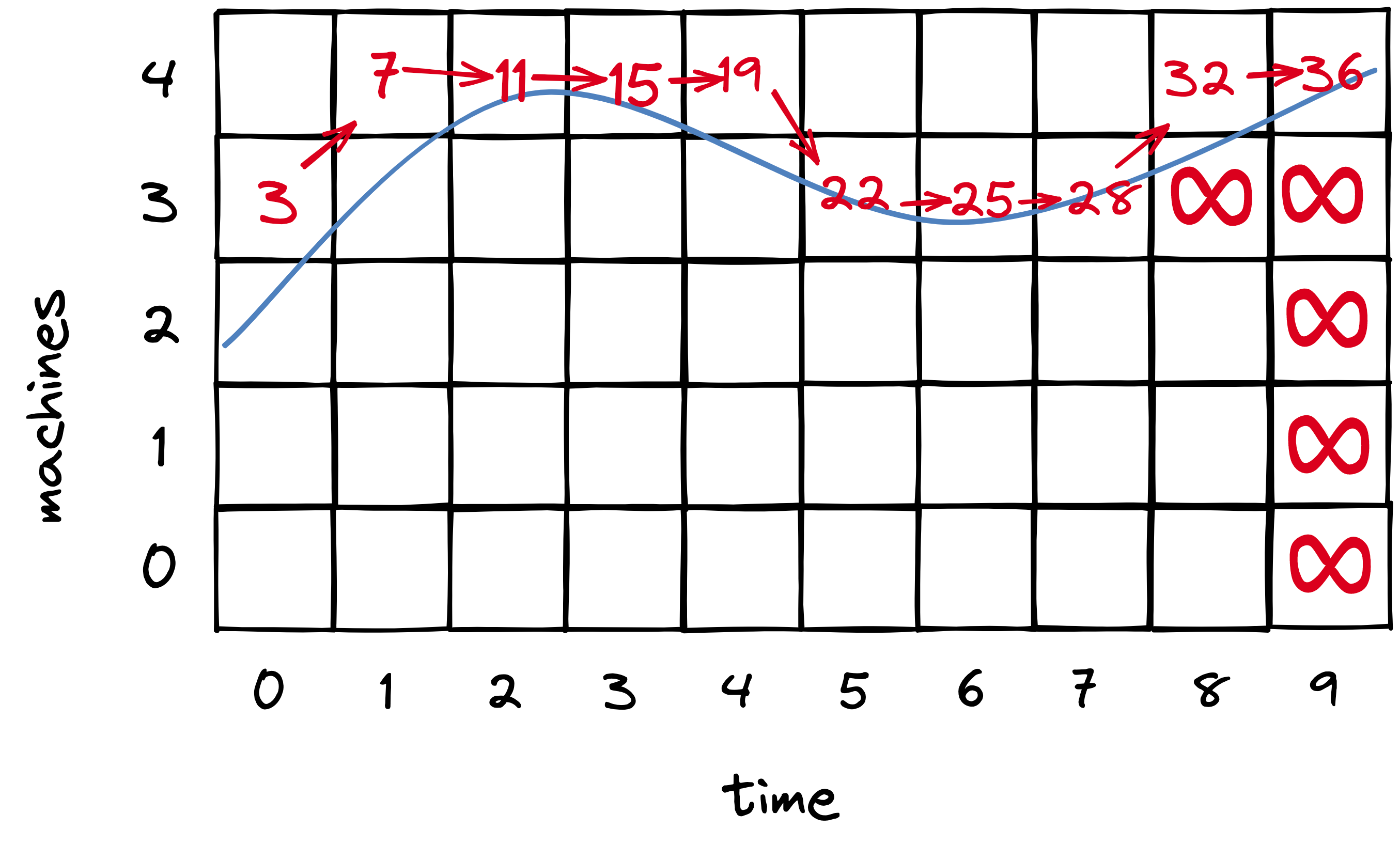
As the planner proceeds up the end-state (rightmost) cells from bottom to top, as soon as it finds a cell with a feasible path to it, the job’s done. Any higher end-state cell would use more machines than necessary.
I hope that explanation made sense, see Taft’s thesis for more. I’m papering over many details: effective capacity is a curve as I showed above, machines are added as late as possible within a step to minimize cost, and some steps are faster than others depending on how parallelizable the data transfers are. The gist is, the planner finds the optimal path using a straightforward algorithm, with a big-O complexity equal to the max number of machines multiplied by the number of future time slots.
P-Store workflow #
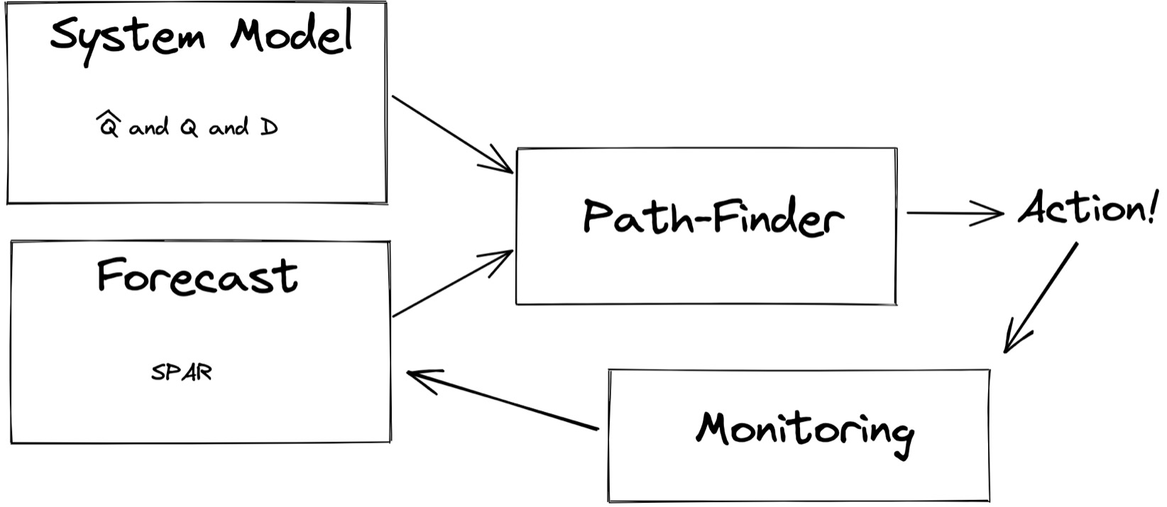
Before deploying the system, humans determine the system model parameters Q̂, Q, and D once, experimentally. (I think a real-world system would have to automatically and frequently update these parameters.) Then, every few minutes, P-Store makes a new forecast based on the latest history, and feeds it into the planner. The planner executes the next step. Continuous monitoring generates new history, which feeds into the next forecast, and so on.
Their evaluation of P-Store #
P-Store is designed with these assumptions:
- The workload mix and data size are not quickly changing. (Because this would make the system model parameters outdated; I think a real-world system could handle these changes by frequently updating Q̂, Q, and D.)
- The workload and data are distributed evenly across the partitions. (Otherwise the system model is inaccurate. Perhaps a combination of E-Store and P-Store, or a more sophisticated system model, could handle skewed load.)
- The workload has few distributed transactions. (Otherwise, moving data could affect the efficiency of transactions. See Clay, which moves data in order to minimize distributed transactions.)
With these simplifying assumptions in place, the authors evaluate how well P-Store meets its goals: avoid latency spikes with minimal cost.
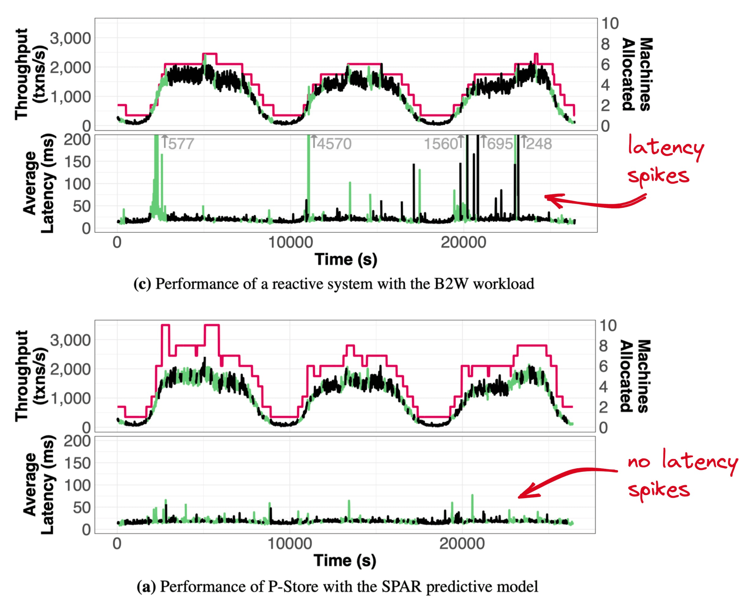
Credit: Taft et al. I added the red arrows.
B2W, the “Amazon of Brazil”, doesn’t actually use P-Store, E-Store, or their foundation H-Store. The authors simulated how it would have performed by replaying 3 days of B2W transactions on E-Store and P-Store. E-Store must scale out while demand is rising (the pink line intersects with green/black line) so it experiences latency spikes. P-Store scales out ahead of rising demand, so it keeps latency low. (P-Store appears to over-allocate; Taft told me this is probably an artifact of the chart resolution. P-Store anticipates abrupt load spikes that are too brief to be visible here.)
My evaluation of P-Store #
- “Workloads are often cyclic, hence predictable” is a great insight, and starting to scale before the spike is brilliant.
- Real-world implementations need not use SPAR or the P-Store path-finding algorithm. The research prototype proved that these particular techniques work well, but they’re not the only possibilities. For me, the overall system concept was more valuable than the details.
- A real world deployment would need some enhancements: It would need to handle skewed workloads, and automatically update Q̂, Q, and D.
Both E-Store and P-Store show straightforward and novel (to me) techniques for autoscaling databases. These ideas were obviously useful in 2017, and even more now: the industry is starting to build serverless databases (including my team at MongoDB), which compete on their efficiency at matching resources to demand. Precise allocation will make the difference between life and death for some companies.